Chapter 1. Introduction to SQL
In this introductory chapter, we explore the origin and utility of the SQL language, demonstrate some of the more useful features of the language, and define a simple database design from which most examples in the book are derived.
What Is SQL?
SQL is a special-purpose language used to define, access, and manipulate data. SQL is nonprocedural, meaning that it describes the necessary components (i.e., tables) and desired results without dictating exactly how those results should be computed. Every SQL implementation sits atop a database engine , whose job it is to interpret SQL statements and determine how the various data structures in the database should be accessed to accurately and efficiently produce the desired outcome.
The SQL language includes two distinct sets of commands: Data Definition Language (DDL) is the subset of SQL used to define and modify various data structures, while Data Manipulation Language (DML) is the subset of SQL used to access and manipulate data contained within the data structures previously defined via DDL. DDL includes numerous commands for handling such tasks as creating tables, indexes, views, and constraints, while DML is comprised of just five statements:
Some people feel that DDL is the sole property of database administrators, while database developers are responsible for writing DML statements, but the two are not so easily separated. It is difficult to efficiently access and manipulate data without an understanding of what data structures are available and how they are related; likewise, it is difficult to design appropriate data structures without knowledge of how the data will be accessed. That being said, this book deals almost exclusively with DML, except where DDL is presented to set the stage for one or more DML examples. The reasons for focusing on just the DML portion of SQL include:
DDL is well represented in various books on database design and administration as well as in SQL reference guides.
Most database performance issues are the result of inefficient DML statements.
Even with a paltry five statements, DML is a rich enough topic to warrant not just one book, but a whole series of books.
Tip
Anyone who writes SQL in an Oracle environment should be armed with the following three books: a reference guide to the SQL language, such as Oracle in a Nutshell (O’Reilly); a performance-tuning guide, such as Optimizing Oracle Performance (O’Reilly); and the book you are holding, which shows how to best utilize and combine the various features of Oracle’s SQL implementation.
So why should you care about SQL? In this age of Internet computing and n-tier architectures, does anyone even care about data access anymore? Actually, efficient storage and retrieval of information is more important than ever:
Many companies now offer services via the Internet. During peak hours, these services may need to handle thousands of concurrent requests, and unacceptable response times equate to lost revenue. For such systems, every SQL statement must be carefully crafted to ensure acceptable performance as data volumes increase.
We can store a lot more data today than we could just a few years ago. A single disk array can hold tens of terabytes of data, and the ability to store hundreds of terabytes is just around the corner. Software used to load or analyze data in these environments must harness the full power of SQL to process ever-increasing data volumes within constant (or shrinking) time windows.
Hopefully, you now have an appreciation for what SQL is and why it is important. The next section will explore the origins of the SQL language and the support for the SQL standard in Oracle’s products.
A Brief History of SQL
In the early 1970s, an IBM research fellow named Dr. E. F. Codd endeavored to apply the rigors of mathematics to the then-untamed world of data storage and retrieval. Codd’s work led to the definition of the relational data model and a language called DSL/Alpha for manipulating data in a relational database. IBM liked what they saw, so they commissioned a project called System/R to build a prototype based on Codd’s work. Among other things, the System/R team developed a simplified version of DSL called SQUARE, which was later renamed SEQUEL, and finally renamed SQL.
The work done on System/R eventually led to the release of various IBM products based on the relational model. Other companies, such as Oracle, rallied around the relational flag as well. By the mid 1980s, SQL had gathered sufficient momentum in the marketplace to warrant oversight by the American National Standards Institute (ANSI). ANSI released its first SQL standard in 1986, followed by updates in 1989, 1992, 1999, and 2003. There will undoubtedly be further refinements in the future.
Thirty years after the System/R team began prototyping a relational database, SQL is still going strong. While there have been numerous attempts to dethrone relational databases in the marketplace, well-designed relational databases coupled with well-written SQL statements continue to succeed in handling large, complex data sets where other methods fail.
Oracle’s SQL Implementation
Given that Oracle was an early adopter of the relational model and SQL, one might think that they would have put a great deal of effort into conforming with the various ANSI standards. For many years, however, the folks at Oracle seemed content that their implementation of SQL was functionally equivalent to the ANSI standards without being overly concerned with true compliance. Beginning with the release of Oracle8i, however, Oracle has stepped up its efforts to conform to ANSI standards and has tackled such features as the CASE statement and the left/right/full outer join syntax.
Ironically, the business community seems to be moving in the opposite direction. A few years ago, people were much more concerned with portability and would limit their developers to ANSI-compliant SQL so that they could implement their systems on various database engines. Today, companies tend to pick a database engine to use across the enterprise and allow their developers to use the full range of available options without concern for ANSI-compliance. One reason for this change in attitude is the advent of n-tier architectures, where all database access can be contained within a single tier instead of being scattered throughout an application. Another possible reason might be the emergence of clear leaders in the DBMS market over the last decade, such that managers perceive less risk in which database engine they choose.
Theoretical Versus Practical Terminology
If you were to peruse the various writings on the relational model, you would come across terminology that you will not find used in this book (such as relations and tuples). Instead, we use practical terms such as tables and rows, and we refer to the various parts of a SQL statement by name rather than by function (i.e., “SELECT clause” instead of projection). With all due respect to Dr. Codd, you will never hear the word tuple used in a business setting, and, since this book is targeted toward people who use Oracle products to solve business problems, you won’t find it here either.
A Simple Database
Because this is a practical book, it contains numerous examples. Rather than fabricating different sets of tables and columns for every chapter or section in the book, we have decided to draw from a single, simple schema for most examples. The subject area that we chose to model is a parts distributor, such as an auto-parts wholesaler or medical device distributor, in which the business fills customer orders for one or more parts that are supplied by external suppliers. Figure 1-1 shows the entity-relationship model for this business.
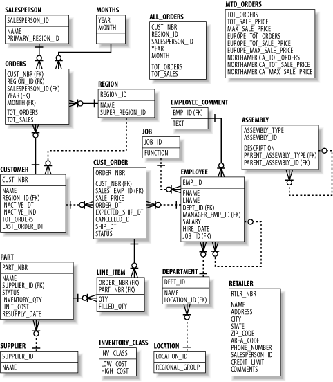
If you are unfamiliar with
entity-relationship
models, here is a brief description of how they work. Each box in the
model represents an entity, which correlates to
a database table.[1] The
lines between the entities represent the
relationships between
tables,
which correlate to foreign keys. For example, the
cust_order table holds a foreign key to the
employee table, which
signifies the salesperson responsible for
a particular order. Physically, this means that the
cust_order table contains a column holding
employee ID numbers, and that, for any given order, the employee ID
number indicates the employee who sold that order. If you find this
confusing, simply use the diagram as an illustration of the tables
and columns found within our database. As you work your way through
the SQL examples in this book, return occasionally to the diagram,
and you should find that the relationships start making sense.
DML Statements
In this section, we will introduce the five statements that comprise the DML portion of SQL. The information presented in this section should be enough to allow you to start writing DML statements. As is discussed at the end of the section, however, DML can look deceptively simple, so keep in mind while reading the section that there are many more facets to DML than are discussed here.
The SELECT Statement
The SELECT statement is used to retrieve data from a database. The set of data retrieved via a SELECT statement is referred to as a result set. Like a table, a result set is comprised of rows and columns, making it possible to populate a table using the result set of a SELECT statement. The SELECT statement can be summarized as follows:
SELECT <one or more things>
FROM <one or more places>
WHERE <zero, one, or more conditions apply>
While the SELECT and FROM clauses are required, the WHERE clause is
optional (although you will seldom see it omitted). We will therefore
begin with a simple example that retrieves three columns from every
row of the
customer table:
SELECT cust_nbr, name, region_idFROM customer;CUST_NBR NAME REGION_ID ---------- ------------------------------ ---------- 1 Cooper Industries 5 2 Emblazon Corp. 5 3 Ditech Corp. 5 4 Flowtech Inc. 5 5 Gentech Industries 5 6 Spartan Industries 6 7 Wallace Labs 6 8 Zantech Inc. 6 9 Cardinal Technologies 6 10 Flowrite Corp. 6 11 Glaven Technologies 7 12 Johnson Labs 7 13 Kimball Corp. 7 14 Madden Industries 7 15 Turntech Inc. 7 16 Paulson Labs 8 17 Evans Supply Corp. 8 18 Spalding Medical Inc. 8 19 Kendall-Taylor Corp. 8 20 Malden Labs 8 21 Crimson Medical Inc. 9 22 Nichols Industries 9 23 Owens-Baxter Corp. 9 24 Jackson Medical Inc. 9 25 Worcester Technologies 9 26 Alpha Technologies 10 27 Phillips Labs 10 28 Jaztech Corp. 10 29 Madden-Taylor Inc. 10 30 Wallace Industries 10
Since we neglected to impose any conditions via a WHERE clause, the query returns every row from the customer table. If you want to restrict the set of data returned by the query, you can include a WHERE clause with a single condition:
SELECT cust_nbr, name, region_idFROM customerWHERE region_id = 8;CUST_NBR NAME REGION_ID ---------- ------------------------------ ---------- 16 Paulson Labs 8 17 Evans Supply Corp. 8 18 Spalding Medical Inc. 8 19 Kendall-Taylor Corp. 8 20 Malden Labs 8
The result set now includes only those customers residing in the
region with a region_id of 8. But what if you want
to specify a region by name instead of region_id?
You could query the region table for a particular
name and then query the customer table using the
retrieved region_id. Instead of issuing two
different queries, however, you can produce the same
outcome using a single query by
introducing a join, as in:
SELECT customer.cust_nbr, customer.name, region.nameFROM customer INNER JOIN regionON region.region_id = customer.region_idWHERE region.name = 'New England';CUST_NBR NAME NAME ---------- ------------------------------ ----------- 1 Cooper Industries New England 2 Emblazon Corp. New England 3 Ditech Corp. New England 4 Flowtech Inc. New England 5 Gentech Industries New England
The FROM clause now contains two tables instead of one and includes a
join condition that specifies that the
customer and region tables are
to be joined using the region_id column found in
both tables. Joins and join conditions will be explored in detail in
Chapter 3.
Since both the customer and
region tables contain a column called
name, you must specify which
table’s name column you are
interested in. This is done in the previous example by using
dot-notation to append the table name in front of each column name.
If you would rather not type full table names, you can assign
table aliases
to each table in the FROM clause and use those aliases instead of the
table names in the SELECT and WHERE clauses, as in:
SELECT c.cust_nbr, c.name, r.name
FROM customer c INNER JOIN region r
ON r.region_id = c.region_id
WHERE r.name = 'New England';
In this example, we assigned the alias c to the
customer table and the alias r to the region
table. Thus, we can use c. and
r. instead of customer. and
region. in the SELECT and WHERE
clauses.
SELECT clause elements
In the examples thus far, the result sets generated by our queries have contained columns from one or more tables. While most elements in your SELECT clauses will typically be simple column references, a SELECT clause may also include:
Literal values, such as numbers (27) or strings (`abc')
Expressions, such as shape.diameter * 3.1415927
Function calls, such as TO_DATE(`01-JAN-2004',`DD-MON-YYYY')
Pseudocolumns, such as ROWID, ROWNUM, or LEVEL
While the first three items in this list are fairly straightforward, the last item merits further discussion. Oracle makes available several phantom columns, known as pseudocolumns , that do not exist in any tables. Rather, they are values visible during query execution that can be helpful in certain situations.
For example, the pseudocolumn ROWID represents the physical location of a row. This information represents the fastest possible access mechanism. It can be useful if you plan to delete or update a row retrieved via a query. However, you should never store ROWID values in the database, nor should you reference them outside of the transaction in which they are retrieved, since a row’s ROWID can change in certain situations, and ROWIDs can be reused after a row has been deleted.
The next example demonstrates each of the different element types from the previous list:
SELECT ROWNUM,cust_nbr,1 multiplier,'cust # ' || cust_nbr cust_nbr_str,'hello' greeting,TO_CHAR(last_order_dt, 'DD-MON-YYYY') last_orderFROM customer;ROWNUM CUST_NBR MULTIPLIER CUST_NBR_STR GREETING LAST_ORDER ------ -------- ---------- ------------ -------- ----------- 1 1 1 cust # 1 hello 15-JUN-2000 2 2 1 cust # 2 hello 27-JUN-2000 3 3 1 cust # 3 hello 07-JUL-2000 4 4 1 cust # 4 hello 15-JUL-2000 5 5 1 cust # 5 hello 01-JUN-2000 6 6 1 cust # 6 hello 10-JUN-2000 7 7 1 cust # 7 hello 17-JUN-2000 8 8 1 cust # 8 hello 22-JUN-2000 9 9 1 cust # 9 hello 25-JUN-2000 10 10 1 cust # 10 hello 01-JUN-2000 11 11 1 cust # 11 hello 05-JUN-2000 12 12 1 cust # 12 hello 07-JUN-2000 13 13 1 cust # 13 hello 07-JUN-2000 14 14 1 cust # 14 hello 05-JUN-2000 15 15 1 cust # 15 hello 01-JUN-2000 16 16 1 cust # 16 hello 31-MAY-2000 17 17 1 cust # 17 hello 28-MAY-2000 18 18 1 cust # 18 hello 23-MAY-2000 19 19 1 cust # 19 hello 16-MAY-2000 20 20 1 cust # 20 hello 01-JUN-2000 21 21 1 cust # 21 hello 26-MAY-2000 22 22 1 cust # 22 hello 18-MAY-2000 23 23 1 cust # 23 hello 08-MAY-2000 24 24 1 cust # 24 hello 26-APR-2000 25 25 1 cust # 25 hello 01-JUN-2000 26 26 1 cust # 26 hello 21-MAY-2000 27 27 1 cust # 27 hello 08-MAY-2000 28 28 1 cust # 28 hello 23-APR-2000 29 29 1 cust # 29 hello 06-APR-2000 30 30 1 cust # 30 hello 01-JUN-2000
Tip
Note that the third through sixth columns have been given column aliases, which are names that you assign to a column. If you are going to refer to the columns in your query by name instead of by position, you will want to assign each column a name that makes sense to you.
Interestingly, a SELECT clause is not required to reference columns from any of the tables in the FROM clause. For example, the next query’s result set is composed entirely of literals:
SELECT 1 num, 'abc' strFROM customer;NUM STR ---------- --- 1 abc 1 abc 1 abc 1 abc 1 abc 1 abc 1 abc 1 abc 1 abc 1 abc 1 abc 1 abc 1 abc 1 abc 1 abc 1 abc 1 abc 1 abc 1 abc 1 abc 1 abc 1 abc 1 abc 1 abc 1 abc 1 abc 1 abc 1 abc 1 abc 1 abc
Since there are 30 rows in the customer table, the
query’s result set includes 30 identical rows of
data.
Ordering your results
In general, there is no guarantee that the result set generated by your query will be in any particular order. If you want your results to be sorted by one or more columns, you can add an ORDER BY clause after the WHERE clause. The following example sorts the results from the New England query by customer name:
SELECT c.cust_nbr, c.name, r.nameFROM customer c INNER JOIN region rON r.region_id = c.region_idWHERE r.name = 'New England'ORDER BY c.name;CUST_NBR NAME NAME -------- ------------------------------ ----------- 1 Cooper Industries New England 3 Ditech Corp. New England 2 Emblazon Corp. New England 4 Flowtech Inc. New England 5 Gentech Industries New England
You may also designate the sort column(s) by their position in the SELECT clause. To sort the previous query by customer number, which is the first column in the SELECT clause, you could issue the following statement:
SELECT c.cust_nbr, c.name, r.nameFROM customer c INNER JOIN region rON r.region_id = c.region_idWHERE r.name = 'New England'ORDER BY 1;CUST_NBR NAME NAME ---------- ------------------------------ ----------- 1 Cooper Industries New England 2 Emblazon Corp. New England 3 Ditech Corp. New England 4 Flowtech Inc. New England 5 Gentech Industries New England
Specifying sort keys by position will certainly save you some typing, but it can often lead to errors if you later change the order of the columns in your SELECT clause.
Removing duplicates
In some cases, your result set may contain duplicate data. For example, if you are compiling a list of parts that were included in last month’s orders, the same part number would appear multiple times if more than one order included that part. If you want duplicates removed from your result set, you can include the DISTINCT keyword in your SELECT clause, as in:
SELECT DISTINCT li.part_nbr
FROM cust_order co INNER JOIN line_item li
ON co.order_nbr = li.order_nbr
WHERE co.order_dt >= TO_DATE('01-JUL-2001','DD-MON-YYYY')
  AND co.order_dt < TO_DATE('01-AUG-2001','DD-MON-YYYY');
This query returns the distinct set of parts ordered during July 2001. Without the DISTINCT keyword, the result set would contain one row for every line-item of every order, and the same part would appear multiple times if it was included in multiple orders. When deciding whether to include DISTINCT in your SELECT clause, keep in mind that finding and removing duplicates necessitates a sort operation, which can greatly increase the execution time of your query.
The INSERT Statement
The INSERT statement is the mechanism for loading data into your database. This section will introduce the traditional single-table INSERT statement, as well as the new multitable INSERT ALL statement introduced in Oracle 9i.
Single-table inserts
With the traditional INSERT statement, data can be inserted into only one
table at a time, although the data being loaded into the table can be
pulled from one or more additional tables. When inserting data into a
table, you do not need to provide values for every column in the
table; however, you need to be aware of the columns that require
non-NULL[2] values and the ones that do not. Here’s
the definition of the employee table:
                  describe employee

Name                                      Null?    Type
----------------------------------------- -------- ------------
EMP_ID                                    NOT NULL NUMBER(5)
FNAME                                              VARCHAR2(20)
LNAME                                              VARCHAR2(20)
DEPT_ID                                   NOT NULL NUMBER(5)
MANAGER_EMP_ID                                     NUMBER(5)
SALARY                                             NUMBER(5)
HIRE_DATE                                          DATE
JOB_ID                                             NUMBER(3)
The NOT NULL designation for the emp_id and
dept_id columns indicates that values are required
for these two columns. Therefore, you must be sure to provide values
for at least these two columns in your INSERT statements, as
demonstrated by the following:
INSERT INTO employee (emp_id, dept_id)
VALUES (101, 20);
Any inserts into employee may optionally include
any or all of the remaining six columns, which are described as
nullable since they may be left undefined. Thus,
you could decide to add the employee’s last name to
the previous statement:
INSERT INTO employee (emp_id, lname, dept_id)
VALUES (101, 'Smith', 20);
The VALUES clause must contain the same number of elements as the
column list, and the data types must match the column definitions. In
this example, emp_id and
dept_id hold numeric values while
lname holds character data, so the INSERT
statement will execute without error. Oracle always tries to convert
data from one type to another automatically, however, so the
following statement will also run without error:
INSERT INTO employee (emp_id, lname, dept_id)
VALUES ('101', 'Smith', '20');
Sometimes, the data to be inserted needs to be retrieved from one or more tables. Since the SELECT statement generates a result set consisting of rows and columns of data, you can feed the result set from a SELECT statement directly into an INSERT statement, as in:
INSERT INTO employee (emp_id, fname, lname, dept_id, hire_date)
SELECT 101, 'Dave', 'Smith', d.dept_id, SYSDATE
FROM department d
WHERE d.name = 'ACCOUNTING';
In this example, the purpose of the SELECT statement is to retrieve
the department ID for the Accounting department. The other four
columns in the SELECT clause are either literals
(101, 'Dave',
'Smith') or function calls (SYSDATE).
Multitable inserts
While inserting data into a single table is the norm, there are
situations where data from a single source must be inserted either
into multiple tables or into the same table multiple times. Such
tasks would normally be handled programatically using PL/SQL, but
Oracle9i introduced the concept of a multitable
insert to allow complex data insertion via a single INSERT statement.
For example, let’s say that one of Mary
Turner’s customers wants to set up a recurring order
on the last day of each month for the next six months. The following
statement adds six rows to the cust_order table
using a SELECT statement that returns exactly one row:
INSERT ALL
INTO cust_order (order_nbr, cust_nbr, sales_emp_id,
  order_dt, expected_ship_dt, status)
VALUES (ord_nbr, cust_nbr, emp_id,
  ord_dt, ord_dt + 7, status)
INTO cust_order (order_nbr, cust_nbr, sales_emp_id,
  order_dt, expected_ship_dt, status)
VALUES (ord_nbr + 1, cust_nbr, emp_id,
  add_months(ord_dt, 1), add_months(ord_dt, 1) + 7, status)
INTO cust_order (order_nbr, cust_nbr, sales_emp_id,
  order_dt, expected_ship_dt, status)
VALUES (ord_nbr + 2, cust_nbr, emp_id,
  add_months(ord_dt, 2), add_months(ord_dt, 2) + 7, status)
INTO cust_order (order_nbr, cust_nbr, sales_emp_id,
  order_dt, expected_ship_dt, status)
VALUES (ord_nbr + 3, cust_nbr, emp_id,
  add_months(ord_dt, 3), add_months(ord_dt, 3) + 7, status)
INTO cust_order (order_nbr, cust_nbr, sales_emp_id,
  order_dt, expected_ship_dt, status)
VALUES (ord_nbr + 4, cust_nbr, emp_id,
  add_months(ord_dt, 4), add_months(ord_dt, 4) + 7, status)
INTO cust_order (order_nbr, cust_nbr, sales_emp_id,
  order_dt, expected_ship_dt, status)
VALUES (ord_nbr + 5, cust_nbr, emp_id,
  add_months(ord_dt, 5), add_months(ord_dt, 5) + 7, status)
SELECT 99990 ord_nbr, c.cust_nbr cust_nbr, e.emp_id emp_id,
  last_day(SYSDATE) ord_dt, 'PENDING' status
FROM customer c CROSS JOIN employee e
WHERE e.fname = 'MARY' and e.lname = 'TURNER'
  and c.name = 'Gentech Industries';
The SELECT statement returns the data necessary for this
month’s order, and the INSERT statement modifies the
order_nbr, order_dt, and
expected_ship_dt columns for the next five
months’ orders. You are not obligated to insert all
rows into the same table, nor must your SELECT statement return only
one row, making the multitable insert statement quite flexible and
powerful. The next example shows how data about a new salesperson can
be entered into both the employee and
salesperson tables:
INSERT ALL
INTO employee (emp_id, fname, lname, dept_id, hire_date)
VALUES (eid, fnm, lnm, did, TRUNC(SYSDATE))
INTO salesperson (salesperson_id, name, primary_region_id)
VALUES (eid, fnm || ' ' || lnm, rid)
SELECT 1001 eid, 'JAMES' fnm, 'GOULD' lnm,
  d.dept_id did, r.region_id rid
FROM department d, region r
WHERE d.name = 'SALES' and r.name = 'Southeast US';
So far, you have seen how multiple rows can be inserted into the same table and how the same rows can be inserted into multiple tables. The next, and final, example of multitable inserts demonstrates how a conditional clause can be used to direct each row of data generated by the SELECT statement into zero, one, or many tables:
INSERT FIRST
  WHEN order_dt < TO_DATE('2001-01-01', 'YYYY-MM-DD') THEN
    INTO cust_order_2000 (order_nbr, cust_nbr, sales_emp_id,
      sale_price, order_dt)
    VALUES (order_nbr, cust_nbr, sales_emp_id, sale_price, order_dt)
  WHEN order_dt < TO_DATE('2002-01-01', 'YYYY-MM-DD') THEN
    INTO cust_order_2001 (order_nbr, cust_nbr, sales_emp_id,
      sale_price, order_dt)
    VALUES (order_nbr, cust_nbr, sales_emp_id, sale_price, order_dt)
  WHEN order_dt < TO_DATE('2003-01-01', 'YYYY-MM-DD') THEN
    INTO cust_order_2002 (order_nbr, cust_nbr, sales_emp_id,
      sale_price, order_dt)
    VALUES (order_nbr, cust_nbr, sales_emp_id, sale_price, order_dt)
SELECT co.order_nbr, co.cust_nbr, co.sales_emp_id,
  co.sale_price, co.order_dt
FROM cust_order co
WHERE co.cancelled_dt IS NULL
  AND co.ship_dt IS NOT NULL;
This statement copies all customer orders prior to January 1, 2003,
to one of three tables depending on the value of the
order_dt column. The keyword FIRST specifies that
once one of the conditions evaluates to TRUE, the statement should
skip the remaining conditions and move on to the next row. If you
specify ALL instead of FIRST, all conditions will be evaluated, and
each row might be inserted into multiple tables if more than one
condition evaluates to TRUE.
The DELETE Statement
The DELETE statement facilitates the removal of data from the database. Like the SELECT statement, the DELETE statement contains a WHERE clause that specifies the conditions used to identify rows to be deleted. If you neglect to add a WHERE clause to your DELETE statement, all rows will be deleted from the target table. The following statement will delete all employees with the last name of Hooper from the employee table:
DELETE FROM employee
WHERE lname = 'HOOPER';
In some cases, the values needed for one or more of the conditions in
your WHERE clause exist in another table. For example, your company
may decide to outsource its accounting functions, thereby
necessitating the removal of all accounting personnel from the
employee table:
DELETE FROM employee
WHERE dept_id =
 (SELECT dept_id
  FROM department
  WHERE name = 'ACCOUNTING');
The use of the SELECT statement in this example is known as a subquery and will be studied in detail in Chapter 5.
In certain cases, you may want to restrict the number of rows that
are to be deleted from a table. For example, you may want to remove
all data from a table, but you want to limit your transactions to no
more than 100,000 rows. If the cust_order table
contained 527,365 records, you would need to find a way to restrict
your DELETE statement to 100,000 rows and then run the statement six
times until all the data has been purged. The following example
demonstrates how the ROWNUM pseudocolumn may be used in a DELETE
statement to achieve the desired effect:
DELETE FROM cust_order
WHERE ROWNUM <= 100000;
COMMIT;
The UPDATE Statement
Modifications to existing data are handled by the UPDATE statement. Like the DELETE statement, the UPDATE statement includes a WHERE clause to specify which rows should be targeted. The following example shows how you might give a 10% raise to everyone making less than $40,000:
UPDATE employee
SET salary = salary * 1.1
WHERE salary < 40000;
If you want to modify more than one column in the table, you have two
choices: provide a set of column/value pairs separated by commas, or
provide a set of columns and a subquery. The following two UPDATE
statements modify the inactive_dt and
inactive_ind columns in the
customer table for any customer who
hasn’t placed an order in the past year:
UPDATE customer
SET inactive_dt = SYSDATE, inactive_ind = 'Y'
WHERE last_order_dt < SYSDATE -- 365;

UPDATE customer
SET (inactive_dt, inactive_ind) =
 (SELECT SYSDATE, 'Y' FROM dual)
WHERE last_order_dt < SYSDATE -- 365;
The subquery in the second example is a bit forced, since it uses a
query against the dual table to build a result set
containing two literals, but it should give you an idea of how you
would use a subquery in an UPDATE statement. In later chapters, you
will see far more interesting uses for subqueries.
The MERGE Statement
There are certain situations,
especially
within Data Warehouse applications, where you may want to either
insert a new row into a table or update an existing row depending on
whether or not the data already exists in the table. For example, you
may receive a nightly feed of parts data that contains both parts
that are known to the system along with parts just introduced by your
suppliers. If a part number exists in the part
table, you will need to update the unit_cost and
status columns; otherwise, you will need to insert
a new row.
While you could write code that reads each record from the feed,
determines whether or not the part number exists in the
part table, and issues either an INSERT or UPDATE
statement, you could instead issue a single MERGE
statement.[3] Assuming that your
data feed has been loaded into the part_stg
staging table, your MERGE statement would look something like the
following:
MERGE INTO part p_dest
USING part_stg p_src
ON (p_dest.part_nbr = p_src.part_nbr)
WHEN MATCHED THEN UPDATE
  SET p_dest.unit_cost = p_src.unit_cost, p_dest.status = p_src.status
WHEN NOT MATCHED THEN INSERT (p_dest.part_nbr, p_dest.name,
  p_dest.supplier_id, p_dest.status,  p_dest.inventory_qty,
  p_dest.unit_cost, p_dest.resupply_date)
  VALUES (p_src.part_nbr, p_src.name,
  p_src.supplier_id, p_src.status, 0, p_src.unit_cost, null);
This statement looks fairly complex, so here is a description of what it is doing:
- Lines 1-3
For each row in the
part_stgtable, see if thepart_nbrcolumn exists in the part table.- Lines 4-5
If it does, then update the matching row in the
parttable using data from thepart_stgtable.- Lines 6-10
Otherwise, insert a new row into the
parttable using the data from thepart_stgtable.
So Why Are There 17 More Chapters?
After reading this chapter, you might think that SQL looks pretty simple (at least the DML portion). At a high level, it is fairly simple, and you now know enough about the language to go write some code. However, you will learn over time that there are numerous ways to arrive at the same end point, and some are more efficient and elegant than others. The true test of SQL mastery is when you no longer have the desire to return to what you were working on the previous year, rip out all the SQL, and recode it. For one of us, it took about nine years to reach that point. Hopefully, this book will help you reach that point in far less time.
While you are reading the rest of the book, you might notice that the majority of examples use SELECT statements, with the remainder somewhat evenly distributed across INSERT, UPDATE, and DELETE statements. This disparity is not indicative of the relative importance of SELECT statements over the other three DML statements; rather, SELECT statements are favored because we can show a query’s result set, which should help you to better understand the query, and because many of the points being made using SELECT statements can be applied to UPDATE and DELETE statements as well.
[1] Depending on the purpose of the model, entities may or may not correlate to database tables. For example, a logical model depicts business entities and their relationships, whereas a physical model illustrates tables and their primary/foreign keys. The model in Figure 1-1 is a physical model.
[3] MERGE was introduced in Oracle9i.
Get Mastering Oracle SQL, 2nd Edition now with the O’Reilly learning platform.
O’Reilly members experience books, live events, courses curated by job role, and more from O’Reilly and nearly 200 top publishers.

