Mining the Social Web

Constructing Friendship Graphs

This chapter has used sets as the primary data structure for storing and manipulating data because we’ve primarily been manipulating collections of items such as ID values, and set operations have provided some powerful operations in exchange for very little effort. While there are usually a few general-purpose tools that work fairly well for most jobs, there aren’t any tools that work well for every job. You have a price to pay either way; generally speaking, the price is either paid up front, when you store the data in special indexes (as you learned was the case with CouchDB in the previous chapter), or at query time, when you look it up and don’t have the benefit of those indexes. If you really must have it both ways, you end up paying for it in terms of redundant storage and the complexities associated with denormalization of the data—not to mention the maintenance of the source code itself.

When you start asking questions that lend themselves to a network topology, you may want to export your Redis data into a graph database such as NetworkX (introduced back in Chapter 1). There are many possible graphs you could construct, but let’s assume you’re interested in analyzing the friendships that exist in someone’s social network, so you want a graph indicating which people are friends with one another. Given that social graphs provide tremendous insight and that Example 4-8 already provides the machinery for crawling Twitter relationships, take some time to harvest friendship data for one or more interesting Twitterers. The remainder of this section introduces some examples for analyzing it.

Assuming you’ve harvested friendship data and stored it away in Redis, Example 4-10 demonstrates how to construct a graph of all the common friendships that exist for a user. Basically, you just systematically walk over all the users in a nested loop and create edges whenever a friendship exists between any two people in the universe being considered. Once the data is available to NetworkX, you suddenly have a full arsenal of graph algorithms and utilities at your fingertips. The next section investigates a few of the valuable things you can mine out of a friendship graph.

Example 4-10. Exporting friend/follower data from Redis to NetworkX for easy graph analytics (friends_followers__redis_to_networkx.py)

# -*- coding: utf-8 -*-

# Summary: Build up a digraph where an edge exists between two users 
# if the source node is following the destination node

import os
import sys
import json
import networkx as nx
import redis

from twitter__util import getRedisIdByScreenName
from twitter__util import getRedisIdByUserId

SCREEN_NAME = sys.argv[1]

g = nx.Graph()
r = redis.Redis()

# Compute all ids for nodes appearing in the graph

friend_ids = list(r.smembers(getRedisIdByScreenName(SCREEN_NAME, 'friend_ids')))
id_for_screen_name = json.loads(r.get(getRedisIdByScreenName(SCREEN_NAME,
                                'info.json')))['id']
ids = [id_for_screen_name] + friend_ids

for current_id in ids:
    print >> sys.stderr, 'Processing user with id', current_id

    try:
        current_info = json.loads(r.get(getRedisIdByUserId(current_id, 
                                  'info.json')))
        current_screen_name = current_info['screen_name']
        friend_ids = list(r.smembers(getRedisIdByScreenName(current_screen_name,
                          'friend_ids')))

        # filter out ids for this person if they aren't also SCREEN_NAME's friends too, 
        # which is the basis of the query

        friend_ids = [fid for fid in friend_ids if fid in ids]
    except Exception, e:
        print >> sys.stderr, 'Skipping', current_id

    for friend_id in friend_ids:
        try:
            friend_info = json.loads(r.get(getRedisIdByUserId(friend_id,
                                     'info.json')))
        except TypeError, e:
            print >> sys.stderr, '\tSkipping', friend_id, 'for', current_screen_name
            continue

        g.add_edge(current_screen_name, friend_info['screen_name'])

# Pickle the graph to disk...

if not os.path.isdir('out'):
    os.mkdir('out')

filename = os.path.join('out', SCREEN_NAME + '.gpickle')
nx.write_gpickle(g, filename)

print 'Pickle file stored in: %s' % filename

# You can un-pickle like so...

# g = nx.read_gpickle(os.path.join('out', SCREEN_NAME + '.gpickle'))

With the task of constructing a convenient graph representation from the friendships you’ve crawled and stored in Redis, let’s now turn to the fun part: analyzing it.

Clique Detection and Analysis

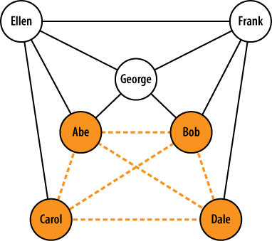
Example 4-10 provides a terse routine that demonstrates how you might go about discovering friendship cliques that exist for a given user by importing data from Redis and repeatedly adding edges to the graph via the idempotent add_edge operation. For example, if Abe is friends with Bob, Carol, and Dale, and Bob and Carol are also friends, the largest (“maximum”) clique in the graph exists among Abe, Bob, and Carol. If Abe, Bob, Carol, and Dale were all mutual friends, however, the graph would be fully connected, and the maximum clique would be of size 4. Adding nodes to the graph might create additional cliques, but it would not necessarily affect the size of the maximum clique in the graph. In the context of the social web, cliques are fascinating because they are representative of mutual friendships, and the maximum clique is interesting because it indicates the largest set of common friendships in the graph. Given two social networks, comparing the sizes of the maximum friendship cliques might provide a lot of insight about group dynamics, among other things.

Figure 4-2 illustrates a sample graph with the maximum clique highlighted. This graph would be said to have a clique number of size 4.

Note

Technically speaking, there is a difference between a maximal clique and a maximum clique. The maximum clique is the largest clique in the graph (or cliques in the graph, if they have the same size). A maximal clique, on the other hand, is one that is not a subgraph of another clique. The maximum clique is also a maximal clique in that it isn’t a subgraph of any other clique. However, various other maximal cliques often exist in graphs and need not necessarily share any nodes with the maximum clique. Figure 4-2, for example, illustrates a maximum clique of size 4, but there are several other maximal cliques of size 3 in the graph as well.

Finding cliques is an NP-complete problem (implying an exponential runtime), but NetworkX does provide the find_cliques method, which delivers a solid implementation that takes care of the heavy lifting. Just be advised that it might take a long time to run as graphs get beyond a reasonably small size.

Figure 4-2. An example graph containing a maximum clique of size 4

Example 4-11 could be modified in any number of ways to compute interesting things, so long as you’ve first harvested the necessary friendship information. Assuming you’ve first constructed a graph as demonstrated in the previous section, it shows you how to use some of the NetworkX APIs for finding and analyzing cliques.

Example 4-11. Using NetworkX to find cliques in graphs (friends_followers__clique_analysis.py)

# -*- coding: utf-8 -*-

import sys
import json
import networkx as nx

G = sys.argv[1]

g = nx.read_gpickle(G)

# Finding cliques is a hard problem, so this could
# take awhile for large graphs.
# See http://en.wikipedia.org/wiki/NP-complete and 
# http://en.wikipedia.org/wiki/Clique_problem

cliques = [c for c in nx.find_cliques(g)]

num_cliques = len(cliques)

clique_sizes = [len(c) for c in cliques]
max_clique_size = max(clique_sizes)
avg_clique_size = sum(clique_sizes) / num_cliques

max_cliques = [c for c in cliques if len(c) == max_clique_size]

num_max_cliques = len(max_cliques)

max_clique_sets = [set(c) for c in max_cliques]
people_in_every_max_clique = list(reduce(lambda x, y: x.intersection(y),
                                  max_clique_sets))

print 'Num cliques:', num_cliques
print 'Avg clique size:', avg_clique_size
print 'Max clique size:', max_clique_size
print 'Num max cliques:', num_max_cliques
print
print 'People in all max cliques:'
print json.dumps(people_in_every_max_clique, indent=4)
print
print 'Max cliques:'
print json.dumps(max_cliques, indent=4)

Sample output from the script follows for Tim O’Reilly’s 600+ friendships and reveals some interesting insights. There are over 750,000 total cliques in the network, with an average clique size of 14 and a maximum clique size of 26. In other words, the largest number of people who are fully connected among Tim’s friends is 26, and there are 6 distinct cliques of this size, as illustrated in the sample output in Example 4-12. The same individuals account for 20/26 of the population in all 6 of those cliques. You might think of these members as being especially foundational for Tim’s friend network. Generally speaking, being able to discover cliques (especially maximal cliques and the maximum clique) in graphs can yield extremely powerful insight into complex data. An analysis of the similarity/diversity of tweet content among members of a large clique would be a very worthy exercise in tweet analysis. (More on tweet analysis in the next chapter.)

Example 4-12. Sample output from Example 4-11, illustrating common members of maximum cliques

Num cliques: 762573
Avg clique size: 14
Max clique size: 26
Num max cliques: 6

People in all max cliques:
[
    "kwerb", 
    "johnbattelle", 
    "dsearls", 
    "JPBarlow", 
    "cshirky", 
    "leolaporte", 
    "MParekh", 
    "mkapor", 
    "steverubel", 
    "stevenbjohnson", 
    "LindaStone", 
    "godsdog", 
    "Joi", 
    "jayrosen_nyu", 
    "dweinberger", 
    "timoreilly", 
    "ev", 
    "jason_pontin", 
    "kevinmarks", 
    "Mlsif"
]

Max cliques:
[
    [
        "timoreilly", 
        "anildash", 
        "cshirky", 
        "ev", 
        "pierre", 
        "mkapor", 
        "johnbattelle", 
        "kevinmarks", 
        "MParekh", 
        "dsearls", 
        "kwerb", 
        "Joi", 
        "LindaStone", 
        "dweinberger", 
        "SteveCase", 
        "leolaporte", 
        "steverubel", 
        "Borthwick", 
        "godsdog", 
        "edyson", 
        "dangillmor", 
        "Mlsif", 
        "JPBarlow", 
        "stevenbjohnson", 
        "jayrosen_nyu", 
        "jason_pontin"
    ], 
     
    ...

    ]

Clearly, there’s much more we could do than just detect the cliques. Plotting the locations of people involved in cliques on a map to see whether there’s any correlation between tightly connected networks of people and geographic locale, and analyzing information in their profile data and/or tweet content are among the possibilities. As it turns out, the next chapter is all about analyzing tweets, so you might want to revisit this idea once you’ve read it. But first, let’s briefly investigate an interesting Web API from Infochimps that we might use as a sanity check for some of the analysis we’ve been doing.

The Infochimps “Strong Links” API

Infochimps is an organization that provides an immense data catalog. Among its many offerings is a huge archive of historical Twitter data and various value-added APIs to operate on that data. One of the more interesting Twitter Metrics and Analytics APIs is the Strong Links API, which returns a list of the users with whom the queried user communicates most frequently. In order to access this API, you just need to sign up for a free account to get an API key and then perform a simple GET request on a URL. The only catch is that the results provide user ID values, which must be resolved to screen names to be useful.^[28] Fortunately, this is easy enough to do using existing code from earlier in this chapter. The script in Example 4-13 demonstrates how to use the Infochimps Strong Links API and uses Redis to resolve screen names from user ID values.

Example 4-13. Grabbing data from the Infochimps Strong Links API (friends_followers__infochimps_strong_links.py)

# -*- coding: utf-8 -*-

import sys
import urllib2
import json
import redis

from twitter__util import getRedisIdByUserId

SCREEN_NAME = sys.argv[1]
API_KEY = sys.argv[2]
API_ENDPOINT = \
    'http://api.infochimps.com/soc/net/tw/strong_links.json?screen_name=%s&apikey=%s'

r = redis.Redis()  # default connection settings on localhost

try:
    url = API_ENDPOINT % (SCREEN_NAME, API_KEY)
    response = urllib2.urlopen(url)
except urllib2.URLError, e:
    print 'Failed to fetch ' + url
    raise e

strong_links = json.loads(response.read())

# resolve screen names and print to screen:

print "%s's Strong Links" % (SCREEN_NAME, )
print '-' * 30
for sl in strong_links['strong_links']:
    if sl is None:
        continue

    try:
        user_info = json.loads(r.get(getRedisIdByUserId(sl[0], 'info.json')))
        print user_info['screen_name'], sl[1]
    except Exception, e:
        print >> sys.stderr, "ERROR: couldn't resolve screen_name for", sl
        print >> sys.stderr, "Maybe you haven't harvested data for this person yet?"

What’s somewhat interesting is that of the 20 individuals involved in all 6 of Tim’s maximum cliques, only @kevinmarks appears in the results set. This seems to imply that just because you’re tightly connected with friends on Twitter doesn’t necessarily mean that you directly communicate with them very often. However, skipping ahead a chapter, you’ll find in Table 5-2 that several of the Twitterers Tim retweets frequently do appear in the strong links list—namely, @ahier, @gnat, @jamesoreilly, @pahlkadot, @OReillyMedia, and @monkchips. (Note that @monkchips is second on the list of strong links, as shown in Example 4-14.) Infochimps does not declare exactly what the calculation is for its Strong Links API, except to say that it is built upon actual tweet content, analysis of which is the subject of the next chapter. The lesson learned here is that tightly connected friendship on Twitter need not necessarily imply frequent communication. (And, Infochimps provides interesting APIs that are definitely worth a look.)

Example 4-14. Sample results from the Infochimps Strong Links API from Example 4-13

timoreilly's Strong Links
------------------------------
jstan 20.115004
monkchips 11.317813
govwiki 11.199023
ahier 10.485066
ValdisKrebs 9.384349
SexySEO 9.224745
tdgobux 8.937282
Scobleizer 8.406802
cheeky_geeky 8.339885
seanjoreilly 8.182084
pkedrosky 8.154991
OReillyMedia 8.086607
FOSSwiki 8.055233
n2vip 8.052422
jamesoreilly 8.015188
pahlkadot 7.811676
ginablaber 7.763785
kevinmarks 7.7423387
jcantero 7.64023
gnat 7.6349654
KentBottles 7.40848
Bill_Romanos 7.3629074
make 7.326427
carlmalamud 7.3147154
rivenhomewood 7.276802
webtechman 7.1044493

Interactive 3D Graph Visualization

It’s a bit out of scope to take a dive into graph-layout algorithms, but it’s hard to pass up an opportunity to introduce Ubigraph, a 3D interactive graph-visualization tool. While there’s not really any analytical value in visualizing a clique, it’s nonetheless a good exercise to learn the ropes. Ubigraph is trivial to install and comes with bindings for a number of popular programming languages, including Python. Example 4-15 illustrates an example usage of Ubigraph for graphing the common members among the maximum cliques for a network. The bad news is that this is one of those opportunities where Windows folks will probably need to consider running a Linux-based virtual machine, since it is unlikely that there will be a build of the Ubigraph server anytime soon. The good news is that it’s not very difficult to pull this together, even if you don’t have advanced knowledge of Linux.

Example 4-15. Visualizing graph data with Ubigraph (friends_followers__ubigraph.py)

# -*- coding: utf-8 -*-

import sys
import json
import networkx as nx

# Packaged with Ubigraph in the examples/Python directory
import ubigraph

SCREEN_NAME = sys.argv[1]
FRIEND = sys.argv[2]

g = nx.read_gpickle(SCREEN_NAME + '.gpickle')

cliques = [c for c in nx.find_cliques(g) if FRIEND in c]
max_clique_size = max([len(c) for c in cliques])
max_cliques = [c for c in cliques if len(c) == max_clique_size]

print 'Found %s max cliques' % len(max_cliques)
print json.dumps(max_cliques, indent=4)

U = ubigraph.Ubigraph()
U.clear()
small = U.newVertexStyle(shape='sphere', color='#ffff00', size='0.2')
largeRed = U.newVertexStyle(shape='sphere', color='#ff0000', size='1.0')

# find the people who are common to all cliques for visualization

vertices = list(set([v for c in max_cliques for v in c]))
vertices = dict([(v, U.newVertex(style=small, label=v)) for v in vertices if v
                not in (SCREEN_NAME, FRIEND)])

vertices[SCREEN_NAME] = U.newVertex(style=largeRed, label=SCREEN_NAME)
vertices[FRIEND] = U.newVertex(style=largeRed, label=FRIEND)

for v1 in vertices:
    for v2 in vertices:
        if v1 == v2:
            continue
        U.newEdge(vertices[v1], vertices[v2])

All in all, you just create a graph and add vertices and edges to it. Note that unlike in NetworkX, however, nodes are not defined by their labels, so you do have to take care not to add duplicate nodes to the same graph. The preceding example demonstrates building a graph by iterating through a dictionary of vertices with minor customizations so that some nodes are easier to see than others. 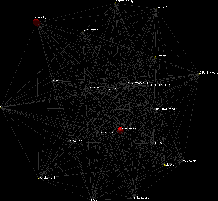Following the pattern of the previous examples, this particular listing would visualize the common members of the maximum cliques shared between a particular user (Tim O’Reilly, in this case) and a friend (defined by FRIEND)—in other words, the largest clique containing two constrained nodes. Figure 4-3 shows a screenshot of Ubigraph at work. Like most everything else in this book, this is just the bare minimum of an introduction, intended to inspire you to go out and do great things with data.

Figure 4-3. Screenshot of an interactive 3D visualization of common members appearing in the maximal cliques containing both @timoreilly and @mikeloukides (the screen shot doesn’t do it justice; you really need to try this out interactively!)

---

^[28] An Infochimps “Who Is” API is forthcoming and will provide a means of resolving screen names from user IDs.