Chapter 1. Introduction to MPLS and SDN
This chapter introduces the basic Multiprotocol Label Switching (MPLS) and Software-Defined Networking (SDN) concepts. These technologies were born for a reason, and a very good way to put them in the proper context is to understand their history. For example, although MPLS has countless applications and use cases today, it was originally conceived to solve a very specific problem in the Internet.
The Internet
The Internet is a collection of autonomous systems (ASs). Each AS is a network operated by a single organization and has routing connections to one or more neighboring ASs.
AS numbers ranging from 64512 to 65534 are reserved for private use. Although the examples in this book use AS numbers from this range, in real life, Internet Service Providers (ISPs) use public AS numbers to peer with their neighboring ASs.
Traditionally, AS numbers were 16 bits (2-byte) long, but newer protocol implementations support AS numbers that are 32 bits (4-byte) in length, too.
Figure 1-1 provides a very simplified view of the Internet. Here, we’re going to take a look at Annika, a random Internet user. She lives in Europe, has a wireline Internet connection at home, and works in a big enterprise that is also connected to the Internet. The company that employs Annika happens to have its own AS number (65001)—this is not a requirement for corporate Internet access. Coincidentally, this company is connected to the Internet through the same ISP (AS 65000) that Annika uses for her residential access.
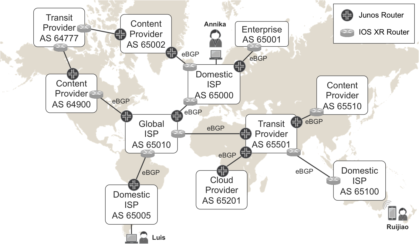
Figure 1-1. The Internet—one day in the life of Annika
As shown in the figure, Annika has two friends who are also ISP subscribers:
-
Ruijiao lives in Oceania and connects with her mobile phone to AS 65100.
-
Luis lives in South America and connects with his laptop to AS 65005.
Annika also uses the public-cloud services of a provider in Africa (65201) and consumes content from different providers in Asia (AS 65510), Europe (AS 65002), and North America (AS 64900).
Figure 1-1 shows different types of providers. The list that follows describes each:
- Domestic ISPs
- In this example, Annika’s residential and corporate Internet connections go through a domestic ISP (AS 65000) that provides Internet access in a particular country, state, or region. Likewise, Ruijiao and Luis are also connected to the Internet through domestic ISPs (AS 65100 and AS 65005, respectively).
- Global ISPs
- 101.230The domestic ISP’s to which Annika (AS 65000) and Luis (AS 65005) are connected belong to the same global ISP group, which has presence in several countries in Europe and America. This global ISP uses a specific network (AS 65010) to interconnect all of the domestic ISPs of the group with one another. In addition, global ISPs also connect their domestic ISPs to the rest of the world.
- Content and cloud providers
- These service providers (SPs) do not generate revenue by charging the subscribers for Internet access. Instead, they provide other types of services to users around the world. For example, they offer multimedia, hosting, cloud services, and so on.
- Transit providers
- These are typically large Tier-1 networks that comprise the Internet skeleton. Their customers are other SPs. If two SPs are not directly connected, they typically reach one another through one or more transit providers.
In practice, this classification is a bit fuzzy. Most SPs try to diversify their portfolios by getting a share from more than one of these markets.
There is yet one more key piece of information in Figure 1-1: the links that interconnect ASs have routers at their endpoints. Pay attention to the icons used for Junos and IOS XR because this convention is used throughout this book.
A router that is placed at the border of an AS and which connects to one or more external ASs is called an AS Border Router (ASBR). Internet ASBRs speak to one another using the Border Gateway Protocol (BGP), described in RFC 4271. BGP runs on top of Transmission Control Protocol (TCP); it is called external BGP (eBGP) if the session’s endpoints are in different ASs. Internet eBGP is responsible for distributing the global IPv4 and IPv6 routing tables. The former already contains more than half a million prefixes and is continually growing.
And this is the Internet some bricks (ASs), links, and a protocol (eBGP) that distributes routing information worldwide. Figure 1-1 is a simplistic representation of the Internet; in reality, it looks more like Figure 1-2.
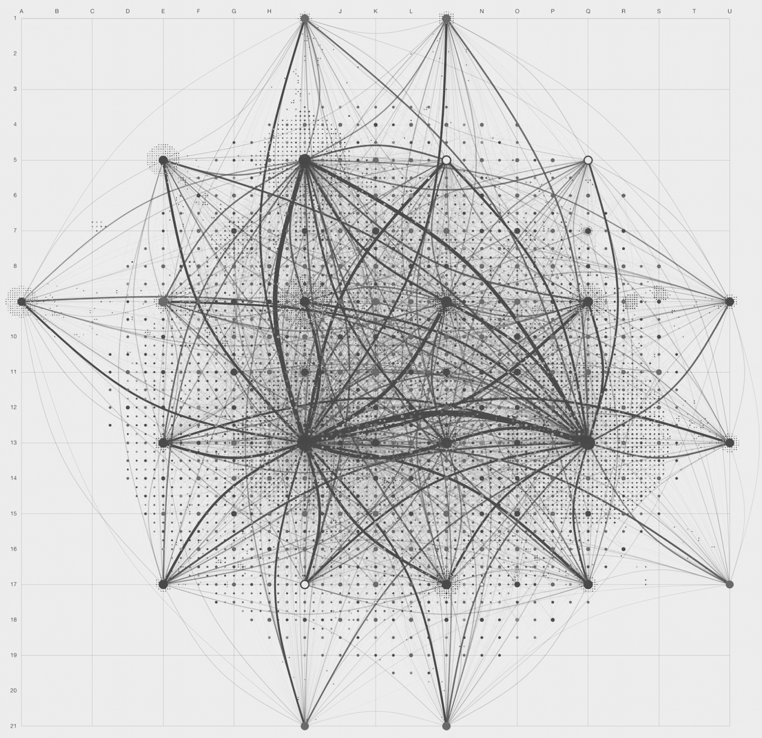
Figure 1-2. The Internet in 2011—topology of autonomous systems (copyright © Peer1 Hosting; used with permission)
This great picture, provided by its owner, Peer1 Hosting, represents ASs as nodes. Peer1’s description of the image is as follows:
This image depicts a graph of 19,869 AS nodes joined by 44,344 connections. The sizing and layout of the ASs is based on their eigenvector centrality, which is a measure of how central to the network each AS is—an AS is central if it is connected to other ASs that are central. This is the same graph-theoretical concept that forms the basis of Google’s PageRank algorithm.
The graph layout begins with the most central nodes and proceeds to the least, positioning them on a grid that subdivides after each order of magnitude of centrality. Within the constraints of the current subdivision level, nodes are placed as near as possible to previously placed nodes that they are connected to.
Note
So far, this description of the Internet is unrelated to MPLS. To understand the original motivation for MPLS, you need to look inside an AS.
Let’s take the time to understand the topology that will be used in the first eight chapters of this book. It is a worthwhile investment of time.
ISP Example Topology
This topology builds on the previous example. Annika is working, and her laptop is H1. At some point, she realizes that she needs to retrieve some data from the provider (more specifically from H3).
Note
For the moment, let’s forget about Network Address Translation (NAT) and imagine that all the addresses are actually public.
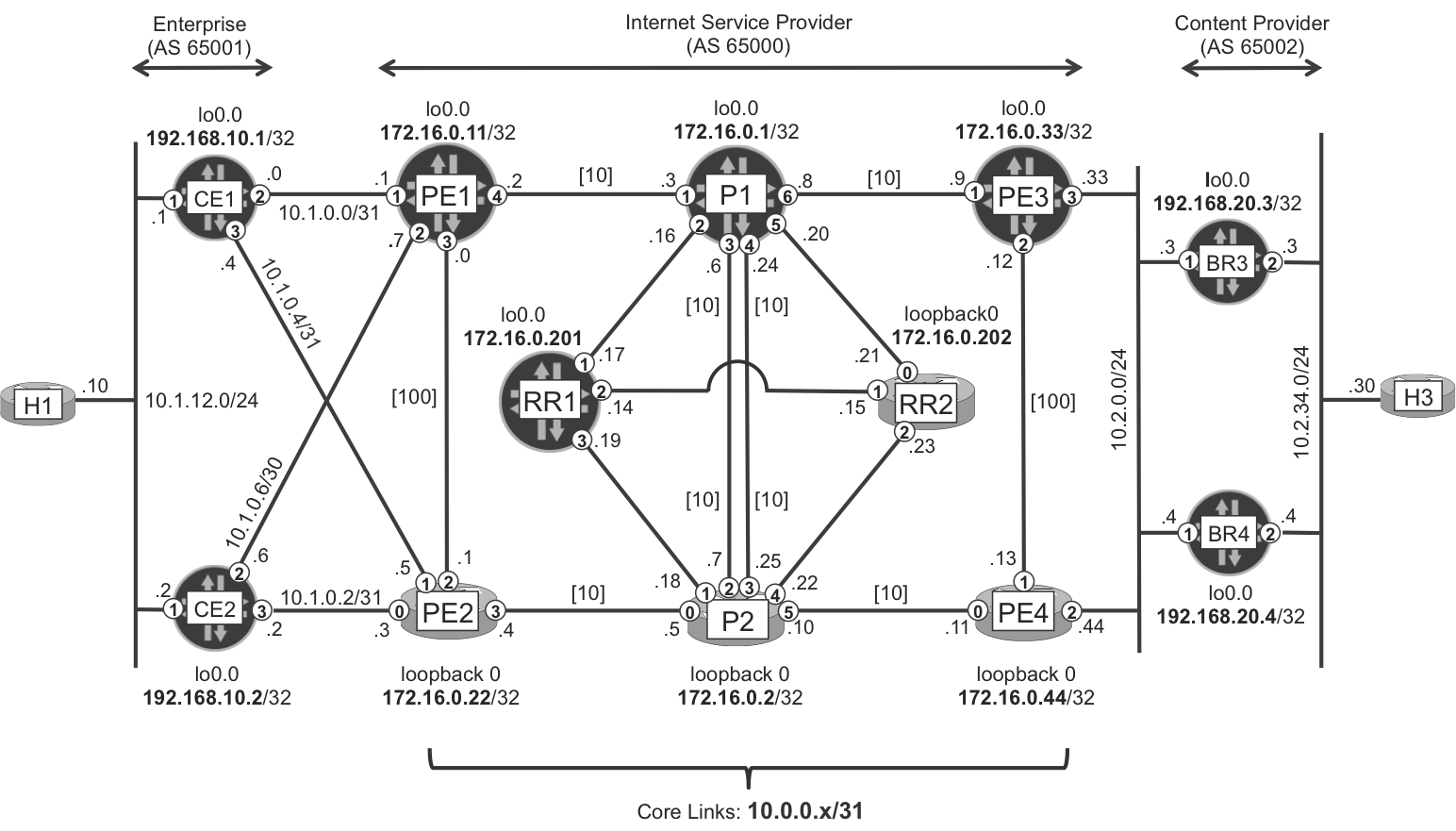
Figure 1-3. Basic ISP topology
More than half of the lab scenarios built for this book run on a single server. The hypervisor spawned virtual machines (VMs) running Junos or IOS XR, which were internally connected through a vSwitch/vRouter.
Around each router, you can see numbers in circles. These are the network interface numbers. For example, if the number inside the circle is <#>, the actual port number is as follows:
-
On devices running Junos, ge-2/0/<#>
-
On devices running IOS XR, Gi 0/0/0/<#>
This convention is used throughout the book.
All the inter-router links are point-to-point (/31), except for the multipoint connection 10.2.0.0/24. Although the latter topology can be found in the WAN access, it is progressively being considered as legacy. For the moment, let’s think of these LANs as classical /24 IPv4 subnets and ignore how they are actually instantiated.
The ISP in this example runs a single Level 2 IS-IS domain with point-to-point interfaces. The PE1-PE2 and PE3-PE4 links are configured with symmetrical IS-IS metric 100, and the remaining core links (PE-P and P-P) are left with the default IS-IS metric 10. These metrics are represented inside square brackets in Figure 1-3.
Warning
Ensure that the RRs are configured with the IS-IS overload bit or with Open Shortest-Path First (OSPF) high metrics so that they do not attract transit traffic.
Router Types in a Service Provider
Although at first sight they look similar, the Enterprise (AS 65001) and the Content Provider (AS 65002) play a different role from the perspective of the ISP (AS 65000):
-
The Enterprise is a corporate customer that pays the ISP for Internet access. It can be dual-homed to more than one ISP for redundancy, but overall the relationship between the Enterprise and the ISP is that of traditional customer-to-provider.
-
The Content Provider has a peering relationship to several ISPs, including AS 65000, AS 64777, and others. The business model is more complex and there is no clear customer-provider relationship: the SPs reach agreements on how to bill for traffic.
The devices in Figure 1-3 play different roles from the perspective of AS 65000, which we’ll explore in the sections that follow.
Customer equipment
CE1 and CE2 in Figure 1-3 are Customer-Premises Equipment (CPE), also known as customer equipment (CE). Traditionally, they are physically located on the customer’s facilities. In the SDN era, it is also possible to virtualize some of their functions and run them on the SP network: this solution is called virtual CPE or vCPE.
For the moment, let’s think of traditional CEs that are on a customer’s network. The operation and management of the CE might be the responsibility of the ISP or the customer, or both. We can classify CEs as follows:
- Residential
- These can be DSL modems, FTTH ONTs, and so on. They don’t run any routing protocols and they are seen by the IP layer of the ISP as directly connected.
- Mobile
- These are smartphones, tablets, and so forth. They also don’t run any routing protocols and are seen by the IP layer of the ISP as directly connected.
- Organizational
- These are dedicated physical or virtual routers that might (or might not) implement an additional set of value-added network functions. They typically have static or dynamic routing to the ISP. eBGP is the most commonly used—and the most scalable—dynamic protocol. If the organization is multihomed to several ISPs, eBGP is simply the only reasonable option.
Note
The organization might be an external enterprise, an internal ISP department, a government institution, a campus, an NGO, and so on.
Now, let’s look at the different functions performed by the core (backbone) routers of the ISP (AS 65000): PE1, PE2, P1, P2, PE3, and PE4.
The core—provider edge
Provider edge (PE) is an edge function performed by ISP-owned core network devices that have both external connections to CEs and internal connections to other core routers. PE1 and PE2 in Figure 1-3 perform the PE role when they forward traffic between CEs and other core routers.
The core—provider
Provider (P) is a core function performed by ISP-owned core routers that have internal backbone connections to more than one other core router. P1 and P2 are pure P-routers because they do not have any connections to external providers or to customers. As for PE1, PE2, PE3, and PE4, they might perform the P role when they forward traffic between two core interfaces. For example, if PE1 receives a packet on ge-2/0/3 and sends it out of ge-2/0/4, it is acting as a P-router.
The border—ASBR
ASBR is an edge function performed by ISP-owned core routers that establish external eBGP peering to other SPs. Although PE1 and PE2 can establish eBGP sessions to CE1 and CE2, they are not considered ASBRs, because the remote peer is a customer, not an SP.
On the other hand, PE3, PE4, BR1, and BR2 are ASBRs, and they perform that function when they forward traffic between external and internal interfaces. For example, if PE3 receives a packet on ge-2/0/1 and sends it out to ge-2/0/3, it is behaving as an ASBR.
The Content Provider (AS 65002) in Figure 1-3 has an overly simplified network. This is fine given that the focus here is on the ISP (AS 65000).
Hosts
The purpose of hosts (H) H1 and H3 in this example is to run ping and traceroute, so their OS is not very relevant. In this example, these hosts are VMs that happen to be running IOS XR; hence, the router icon for a host.
H1 belongs to the customer intranet, and H3 is connected to the content provider core. Neither H1 nor H3 run any routing protocols.
BGP Configuration
Intermediate System–to–Intermediate System (IS-IS) provides loopback-to-loopback connectivity inside the ISP, which is required to establish the multihop internal BGP (iBGP) sessions.
Figure 1-4 shows the BGP sessions and their endpoints: loopback addresses for iBGP, and link addresses on the border (eBGP).
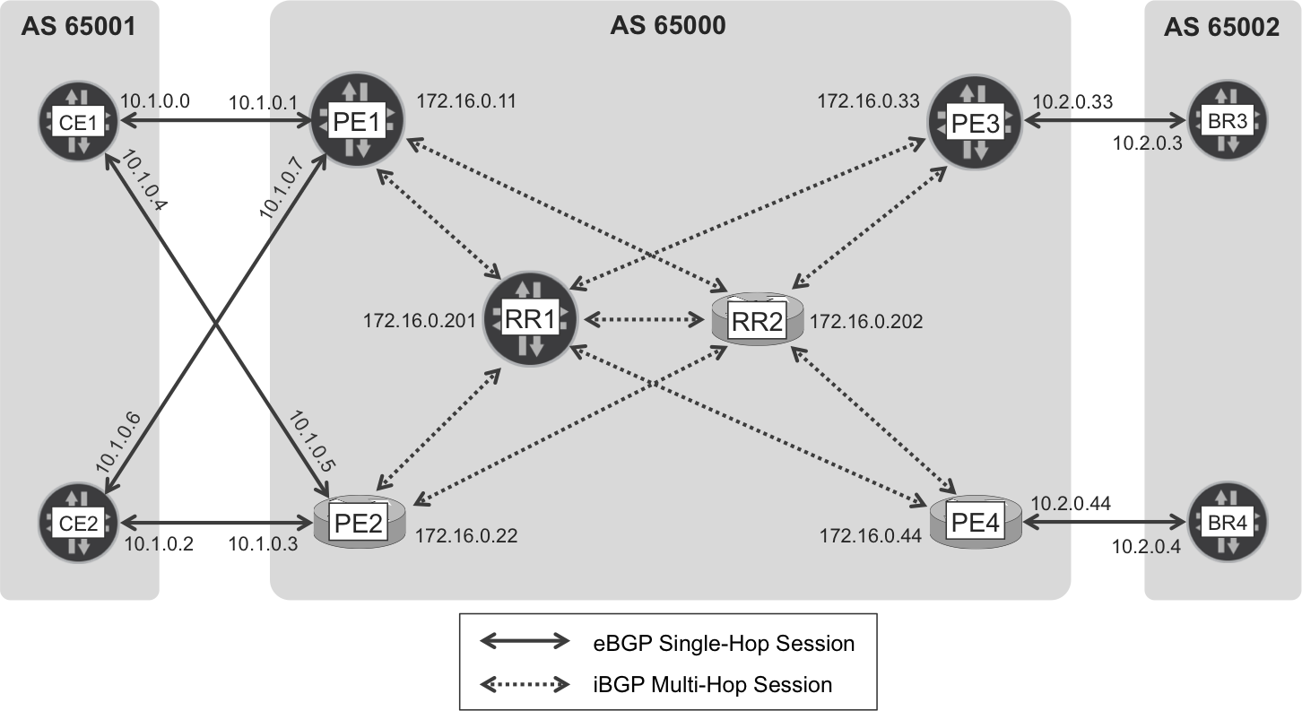
Figure 1-4. Internet eBGP and iBGP sessions
BGP configuration—PEs and ASBRs running Junos
Example 1-1 shows the BGP configuration at PE1.
Example 1-1. BGP configuration at PE1 (Junos)
1     routing-options {
2         autonomous-system 65000;
3     }
4     protocols {
5         bgp {
6             group iBGP-RR {
7                 type internal;
8                 local-address 172.16.0.11;
9                 family inet {
10                    unicast {
11                        add-path {
12                            receive;
13                            send {
14                                path-count 6;
15                            }
16                        }
17                    }
18                }
19                export PL-iBGP-RR-OUT;
20                neighbor 172.16.0.201;
21                neighbor 172.16.0.202;
22            }
23            group eBGP-65001 {
24                family inet {
25                    unicast;
26                }
27                peer-as 65001;
28                neighbor 10.1.0.0 {
29                    export PL-eBGP-65001-CE1-OUT;
30                }
31                neighbor 10.1.0.6 {
32                    export PL-eBGP-65001-CE2-OUT;
33                }
34            }
35        }
36    }
37    policy-options {
38        policy-statement PL-iBGP-RR-OUT {
39            term NHS {
40                from family inet;
41                then {
42                    next-hop self;
43                }
44            }
45        }
46        policy-statement PL-eBGP-65001-CE1-OUT {
47            term BGP {
48                then {
49                    metric 100;
50                }
51            }
52        }
53        policy-statement PL-eBGP-65001-CE2-OUT {
54            term BGP {
55                then {
56                    metric 200;
57                }
58            }
59        }
60    }
PE1 and PE3 have a similar configuration. The different business relationship to the peering providers does not change the fact that the protocol is the same: eBGP.
Lines 6 through 22 contain the loopback-to-loopback configuration for the PE1-RR1 and PE1-RR2 iBGP sessions. The Add-Path functionality (lines 11 through 16) will be explained later.
When a router readvertises a prefix into iBGP, it does not change the original BGP next hop attribute by default. So, if PE1 advertises the 10.1.12.0/24 route to the RRs, the BGP next hop of the route is 10.1.0.0. This next hop is not reachable from inside the ISP—for example, from PE3 and PE4—making the BGP route useless. The cleanest solution is to make PE1 rewrite the BGP next-hop attribute to its own loopback (lines 19, and lines 38 through 45) before advertising the route via iBGP.
Lines 23 through 34 contain the single-hop PE1-CE1 and PE1-CE2 eBGP configuration. The eBGP route policies (lines 29, 32, and 46 through 59) will be explained soon.
BGP configuration—RRs running Junos
This BGP configuration at RR1 is very similar to PE1’s, but it has one key difference, as demonstrated in Example 1-2, for which the neighbors are omitted for brevity.
Example 1-2. BGP configuration at RR1 (Junos)
1     protocols {
2         bgp {
3             group iBGP-CLIENTS {
4                 cluster 172.16.0.201;
5     }}}
What makes RR1 a Route Reflector is line 4; without it, the default iBGP rule—iBGP routes must not be readvertised via iBGP—would apply.
The peering with the other RR (RR2) is configured as a neighbor on a different group that does not contain the cluster statement.
BGP Configuration—PEs and ASBRs running IOS XR
PE2 and PE4 have a similar configuration. Example 1-3 presents that of PE2.
Example 1-3. BGP configuration at PE2 (IOS XR)
1     router bgp 65000
2      address-family ipv4 unicast
3       additional-paths receive
4       additional-paths send
5      !
6      neighbor-group RR
7       remote-as 65000
8       update-source Loopback0
9       address-family ipv4 unicast
10       route-policy PL-iBGP-RR-OUT out
11     !
12     neighbor 10.1.0.2
13      remote-as 65001
14      address-family ipv4 unicast
15       route-policy PL-eBGP-65001-IN in
16       route-policy PL-eBGP-CE2-OUT out
17     !
18     neighbor 10.1.0.4
19      remote-as 65001
20      address-family ipv4 unicast
21       route-policy PL-eBGP-65001-IN in
22       route-policy PL-eBGP-CE1-OUT out
23     !
24     neighbor 172.16.0.201
25      use neighbor-group RR
26     !
27     neighbor 172.16.0.202
28      use neighbor-group RR
29     !
30    !
31    route-policy PL-iBGP-RR-OUT
32      set next-hop self
33    end-policy
34    !
35    route-policy PL-eBGP-CE1-OUT
36      set med 200
37      pass
38    end-policy
39    !
40    route-policy PL-eBGP-CE2-OUT
41      set med 100
42      pass
43    end-policy
44    !
45    route-policy PL-eBGP-65001-IN
46      pass
47    end-policy
The syntax is different, but the principles are very similar to Junos. The Add-Path functionality (lines 3 through 4) will be explained later.
A remarkable difference between the BGP implementation of Junos and IOS XR is that IOS XR by default blocks the reception and advertisement of routes via eBGP. There are two alternative ways to change this default behavior:
-
Explicitly configure input and output policies (lines 15 through 16, 21 through 22, and 35 through 47) in order to allow IOS XR to signal eBGP routes.
-
Configure
router bgp 65000 bgp unsafe-ebgp-policy. This is a shortcut that you can use for quick configuration which is especially useful in the lab. This command automatically creates and attaches the “pass all” policies
Note
Due to the constraints of space, from this point forward, Junos and IOS XR configuration examples may be represented with merged lines.
BGP configuration—RRs running IOS XR
The BGP configuration at RR2 shown in Example 1-4 is very similar to that of PE2, but it has some differences.
Example 1-4. BGP configuration at RR2 (IOS XR)
1     router bgp 65000
2      address-family ipv4 unicast
3       additional-paths receive
4       additional-paths send
5      !
6      neighbor-group iBGP-CLIENTS
7       cluster-id 172.16.0.202
8       address-family ipv4 unicast
9        route-reflector-client
10    !
What makes RR2 a Route Reflector are lines 7 and 9; without them, the default iBGP rule—iBGP routes must not be readvertised via iBGP—would apply.
The peering with the other RR (RR1) is not configured through this neighbor-group.
BGP Route Signaling and Redundancy
This book considers three BGP redundancy models—Nonredundant, Active-Backup, and Active-Active—and they are all supported by the topology in Figure 1-3.
Nonredundant BGP Routes
In this example, CEs and BRs advertise their own loopacks to one single eBGP peer:
-
CE1 advertises 192.168.10.1/32 to PE1 only.
-
CE2 advertises 192.168.10.2/32 to PE2 only.
-
BR3 advertises 192.168.20.3/32 to PE3 only.
-
BR4 advertises 192.168.20.4/32 to PE4 only.
If an eBGP session fails, the loopback of the affected CE or BR is no longer reachable via AS 65000. This scenario is frequent in single-homed access topologies. In this example, it is simulated by selectively blocking the local loopback advertisement from CE1 and CE2 (eBGP export policies), and by only configuring one eBGP session at each BR.
Figure 1-5 shows CE1’s loopback route signaling process.
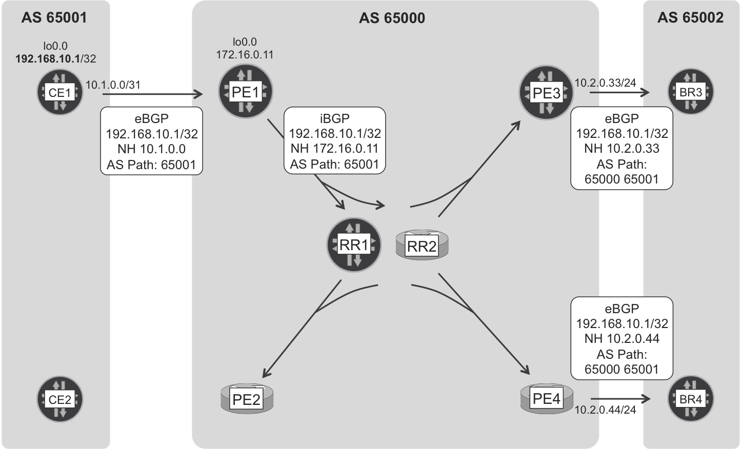
Figure 1-5. Internet eBGP and iBGP route signaling—CE1 loopback
CE1’s loopback is single-homed to PE1, so a packet that any device in AS 65002 sends to CE1’s loopback should go via PE1 at some point.
The RRs do not change the value of the BGP next hop and AS path attributes when they reflect the route to PE2, PE3, and PE4.
On the other hand, PE2 does not advertise the route to CE2, because it would result in an AS loop. This behavior, which you can change by using the as-override configuration command, is further discussed in Chapter 3.
Figure 1-6 shows BR4’s loopback route signaling process.
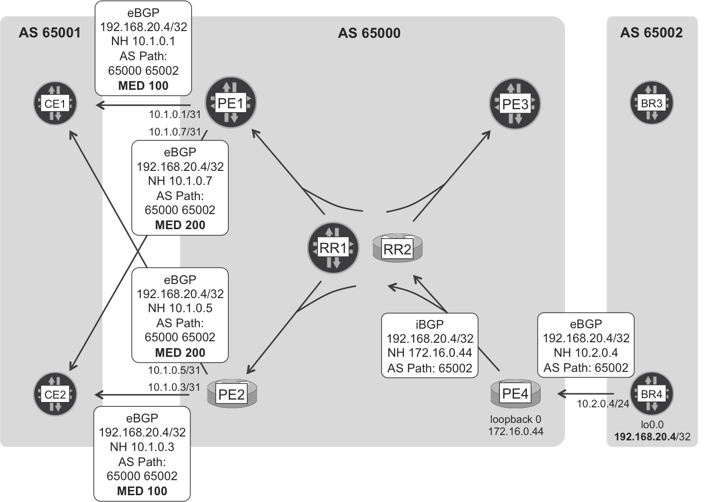
Figure 1-6. Internet eBGP and iBGP route signaling—BR4 loopback
BR4’s loopback is single-homed to PE4, so a packet that any device in AS 65001 sends to BR4’s loopback should go via PE4 at some point.
There is an additional redundancy level on the left side of Figure 1-6. CE1 prefers to reach BR4 via PE1 (Multi Exit Discriminator [MED] 100 is better than MED 200), but if the CE1-PE1 eBGP session fails, it can still fail-over to PE2.
In the absence of access link failures:
Active-Backup BGP routes
As you can see in Figure 1-7, BR3 and BR4 both advertise the 10.2.34.0/24 route, but they do it with a different MED. As a result, PE1 and PE2 prefer to reach BR4 via PE4. If, for whatever reason, PE4 no longer advertises the 10.2.34.0/24 route (or if the route is in an invalid state), then PE1 and PE2 can fail-over to PE3.
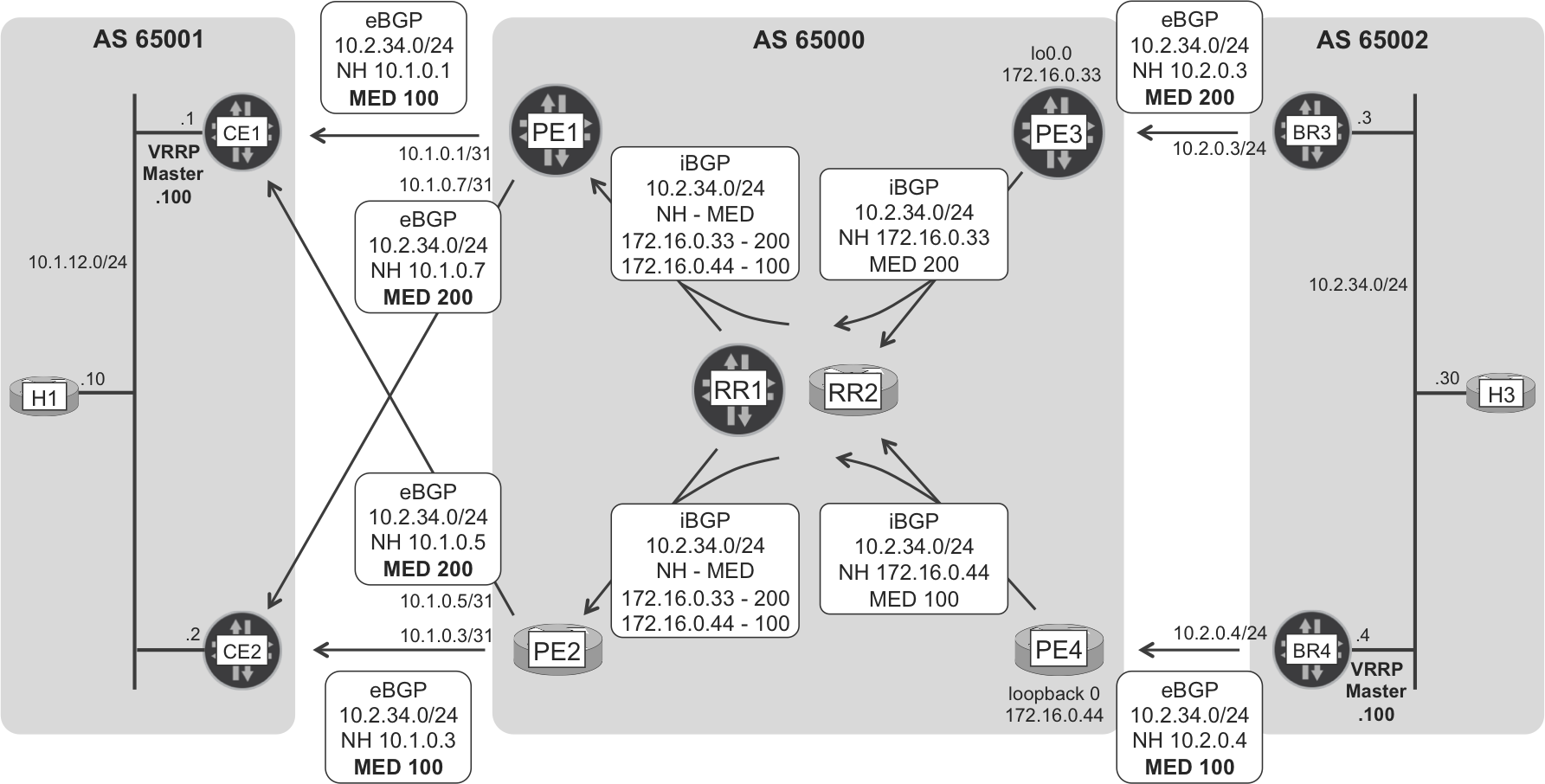
Figure 1-7. Internet eBGP and iBGP route signaling—H3’s subnet
H1 has a default route pointing to the virtual IPv4 address 10.1.12.100. CE1 and CE2 run Virtual Router Redundancy Protocol (VRRP) on the host LAN, and in the absence of failures CE1 is the VRRP master that holds the 10.1.12.100 address. On the other hand, VRRP route tracking is configured so that if CE1 does not have a route to reach H3 and CE2 does, CE2 becomes the VRRP master. The mechanism is very similar between BR3 and BR4, except in this case BR4 is the nominal VRRP master.
Finally, the MED scheme configured on PE1’s and PE2’s eBGP export policies is such that CE1 prefers to reach H3 via PE1 rather than via PE2. With all the links and sessions up, the path followed by H1→H3 (10.1.12.10→10.2.34.30) packets is CE1-PE1-PE4-BR4. VRRP mastership on the first hop, and then MED on the remaining hops, are the tie-breaking mechanisms to choose the best path.
Active-Active BGP routes
PE1 and PE2 both have an eBGP route to 10.1.12.0/24 with MED 100, so both advertise the route with MED 100 to the RRs, as you can see in Figure 1-8.
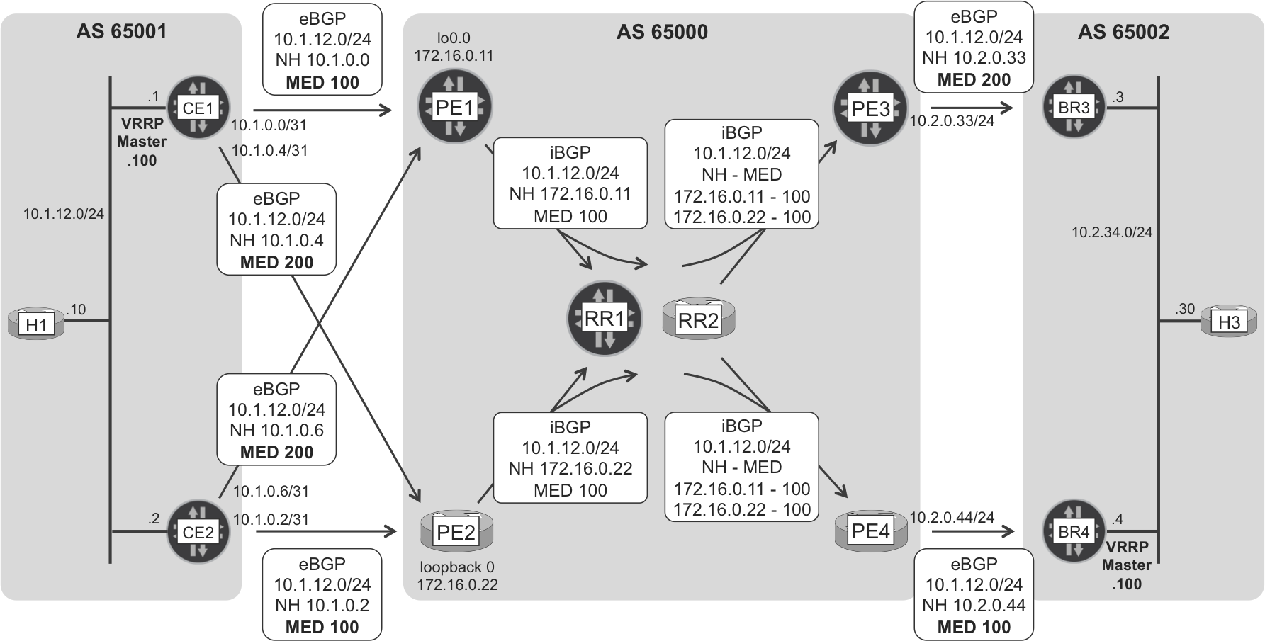
Figure 1-8. Internet eBGP and iBGP route signaling—H1’s subnet
The path followed by H3→H1 packets is BR4-PE4-PE2-CE2. PE4 prefers PE2 because the MED value is 100 for both BGP next hops (PE1 and PE2) and the IGP metric of the shortest internal path PE4→PE2 is lower than the IGP metric of PE4→PE1. Likewise, PE3 prefers PE1, but BR4 is the VRRP master, so PE3 is not in the nominal H3→H1 path.
The end result is asymmetrical but optimal forwarding of H1→H3 and H3→H1 flows. It is optimal because the RRs are reflecting all the routes, not just those that they consider to be the best, as shown in Example 1-5.
Example 1-5. iBGP Route Reflection with Add-Path—RR1 (Junos)
1     juniper@RR1> show route advertising-protocol bgp 172.16.0.44
2                  10.1.12.10
3
4     inet.0: 33 destinations, 38 routes (33 active, ...)
5       Prefix           Nexthop          MED     Lclpref    AS path
6     * 10.1.12.0/24     172.16.0.11      100     100        65001 I
7                        172.16.0.22      100     100        65001 I
8
9     juniper@RR1> show route advertising-protocol bgp 172.16.0.44
10                 10.1.12.0/24 detail
11
12    inet.0: 33 destinations, 38 routes (33 active, ...)
13    * 10.1.12.0/24 (3 entries, 2 announced)
14     BGP group CLIENTS type Internal
15         Nexthop: 172.16.0.11
16         MED: 100
17         Localpref: 100
18         AS path: [65000] 65001 I
19         Cluster ID: 172.16.0.201
20         Originator ID: 172.16.0.11
21         Addpath Path ID: 1
22     BGP group CLIENTS type Internal
23         Nexthop: 172.16.0.22
24         MED: 100
25         Localpref: 100
26         AS path: [65000] 65001 I
27         Cluster ID: 172.16.0.201
28         Originator ID: 172.16.0.22
29         Addpath Path ID: 2
This is possible thanks to the Add-Path extensions (lines 21 and 29). Without them, RR1 would choose the route with the best IGP metric from its own perspective—from the RR to the BGP next hop—which does not necessarily match the perspective from PE4.
In summary, policies are configured in such a way that the MED or BGP metric is symmetrically set. Following are the results:
-
CE1 prefers reaching H3 via PE1 rather than via PE2.
-
CE2 prefers reaching H3 via PE2 rather than via PE1.
-
PE1 prefers reaching H1 via CE1 rather than via CE2.
-
PE2 prefers reaching H1 via CE2 rather than via CE1.
-
PE1 and PE2 prefer reaching H3 via PE4 rather than via PE3.
-
PE3 and PE4 prefer reaching H1 via PE1 and PE2, respectively.
Packet Forwarding in a BGP-Less Core
Everything is fine so far, except for one major detail: H1 and H3 cannot communicate to each other. Let’s take the example of an IPv4 packet with source H1 and destination H3. PE1 decides to forward the packet via PE4, but PE1 and PE4 are not directly connected to each other. The shortest path from PE1 to PE4 is PE1-P1-P2-PE4. Thus, PE1 sends the packet to its next hop, P1. Here is the problem: P1 does not speak BGP, so it does not have a route to the destination H3. As a result, P1 drops the packet.
How about establishing iBGP sessions between P1 and the RRs? This is a relatively common practice in large SPs with high-end core devices. In the real Internet there are more than half a million routes, and it keeps growing. Although route summarization is possible, it still requires a significant control-plane load for P1 to program all the necessary BGP routes. P1 would also lose agility upon network topology changes because it would need to reprogram many routes on the forwarding plane.
P1 and P2 are internal core routers (they do not have any eBGP peerings), and their role is to take packets as fast and reliably as possible between edge routers such as PE1, PE2, PE3, and PE4. This is possible if PE1 adds to the H1→H3 IPv4 packet an extra header—or set of headers—with the following instruction: take me to PE4.
One option is to use IP tunneling. By encapsulating the H1→H3 IPv4 packet inside another IPv4 header with source and destination PE1→PE4, the packet reaches PE4. Then, PE4 removes the tunneling headers and successfully performs an IPv4 lookup on the original H1→H3 packet. There are several IP tunneling technologies available such as GRE, IP-in-IP, and VXLAN. However, this approach has several problems when it comes to forwarding terabits per second or petabits per second, or more.
The most immediate of these problems was cost, given that IP tunneling used to be expensive:
-
First, an IPv4 header alone comprises 20 bytes. Add the extra adaptation headers, and the overhead becomes significant, not to mention the effort that is required to create and destroy headers with many dynamic fields.
-
Second, performing an IPv4 lookup has traditionally been expensive. Although modern platforms have dramatically reduced its differential cost, in the 1990s IPv4 forwarding resulted in a much worse performance than label switching.
There is another technology that is better in terms of overhead (4 bytes per header) and forwarding efficiency. This technology is natively integrated with BGP and brings a large portfolio of features that are of paramount importance to SPs. You might have guessed already that its name is MPLS, or Multiprotocol Label Switching. In the SDN era, forwarding cost is no longer the main driver to deploy MPLS: its architecture and flexibility are.
MPLS
MPLS was invented in the late 1990s, at a time when Asynchronous Transfer Mode (ATM) was a widespread WAN technology.
ATM had some virtues: multiservice, asynchronous transport, class of service, reduced forwarding state, predictability, and so on. But it had at least as many defects: no tolerance to data loss or reordering, a forwarding overhead that made it unsuitable to high speeds, no decent multipoint, lack of a native integration with IP, and so forth.
MPLS learned from the instructive ATM experience, taking advantage of its virtues while solving its defects. Modern MPLS is an asynchronous packet-based forwarding technology. In that sense, it is similar to IP, but MPLS has a much lighter forwarding plane and it greatly reduces the amount of state that needs to be signaled and programmed on the devices.
MPLS in Action
Probably the best way to understand MPLS is by looking at a real example, such as that shown in Figure 1-9.
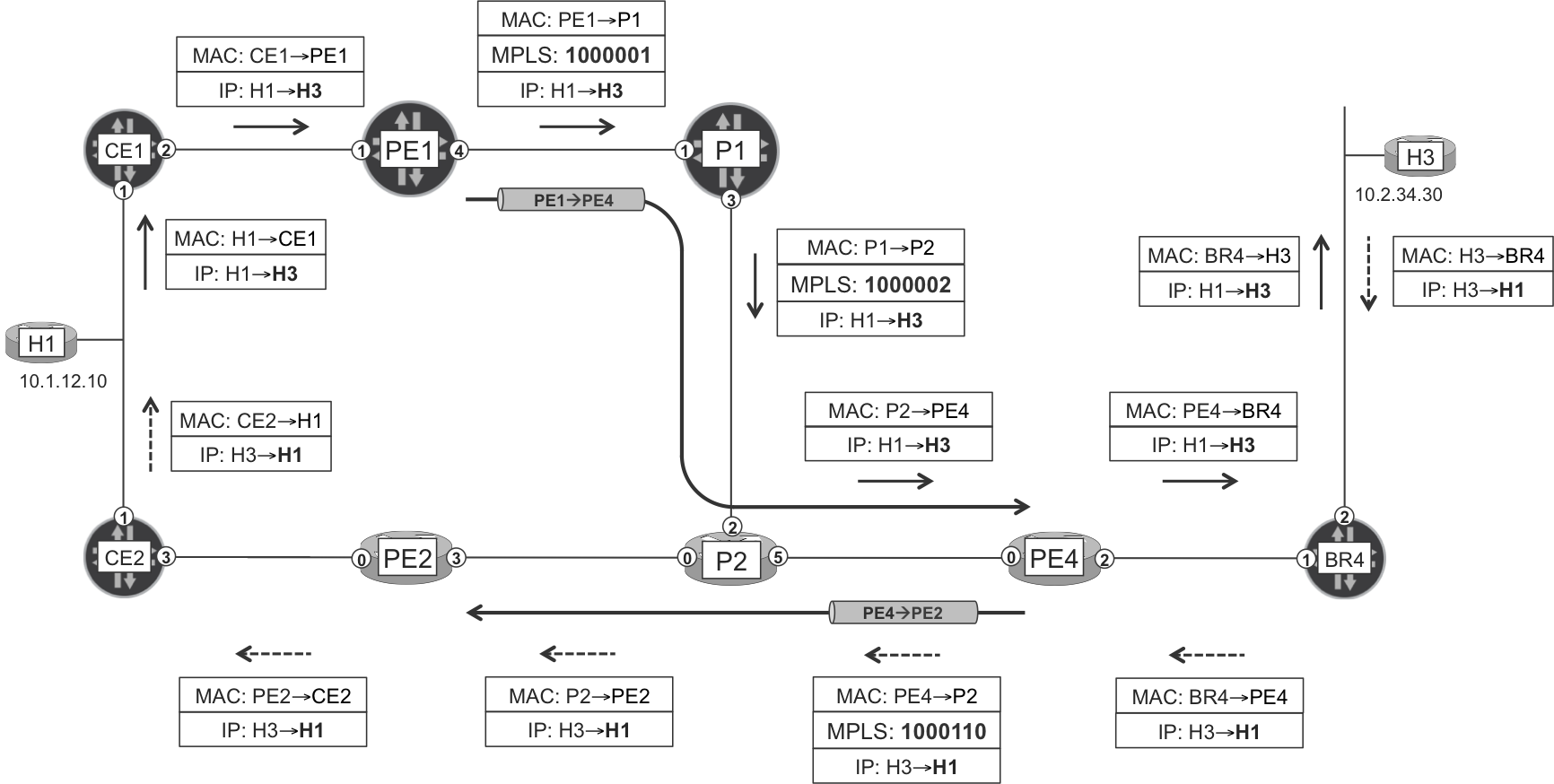
Figure 1-9. MPLS in action
Figure 1-9 shows two unidirectional MPLS Label-Switched Paths (LSPs) named PE1→PE4 and PE4→PE2. Let’s begin with the first one. An IPv4 H1→H3 (10.1.12.10→10.2.34.30) packet arrives at PE1, which leads to the following:
-
H3 is reachable through PE4, so PE1 places the packet in the PE1→PE4 LSP. It does so by inserting a new MPLS header between the IPv4 and the Ethernet headers of the H1→H3 packet. This header contains MPLS label 1000001, which is locally significant to P1. In MPLS terminology, this operation is a label push. Finally, PE1 sends the packet to P1.
-
P1 receives the packet and inspects and removes the original MPLS header. Then, P1 adds a new MPLS header with label 1000002, which is locally significant to P2, and sends the packet to P2. This MPLS operation is called a label swap.
-
P2 receives the packet, inspects and removes the MPLS header, and then sends the plain IPv4 packet to PE4. This MPLS operation is called a label pop.
-
PE4 receives the IPv4 packet without any MPLS headers. This is fine because PE4 speaks BGP and is aware of all the IPv4 routes, so it knows how to forward the packet toward its destination.
The H3→H1 packet travels from PE4 to PE2 in a shorter LSP where only two MPLS operations take place: label push at PE4 and label pop at P2. There is no label swap.
Note
These LSPs happen to follow the shortest IGP path between their endpoints. This is not mandatory and it is often not the case.
Router roles in a LSP
Looking back at Figure 1-9, the PE1→PE4 LSP starts at PE1, traverses P1 and P2, and ends... at P2 or at PE4? Let’s see. By placing the packet in the LSP, PE1 is basically sending it to PE4. Indeed, when P2 receives a packet with label 1000002, the forwarding instruction is clear: pop the label and send the packet out of the interface Gi 0/0/0/5. So the LSP ends at PE4.
Note
The H1→H3 packet arrives unlabeled to PE4 by virtue of a mechanism called Penultimate Hop Popping (PHP) executed by P2.
Following are the different router roles from the point of view of the PE1→PE4 LSP. For each of these roles, there are many terms and acronyms:
-
PE1 Ingress PE, Ingress Label Edge Router (LER), LSP Head-End, LSP Upstream Endpoint. The term ingress comes from the fact that user packets like H1→H3 enter the LSP at PE1, which acts as an entrance or ingress point.
-
P1 (or P2) Transit P, P-Router, Label Switching Router (LSR), or simply P.
-
PE4 Egress PE, Egress Label Edge Router (LER), LSP Tail-End, LSP Downstream Endpoint. The term egress comes from the fact that user packets such as H1→H3 exit the LSP at this PE.
The MPLS Header
Paraphrasing Ivan Pepelnjak, technical director of NIL Data Communications, in his www.ipspace.net blog:
MPLS is not tunneling, it’s a virtual-circuits-based technology, and the difference between the two is a major one. You can talk about tunneling when a protocol that should be lower in the protocol stack gets encapsulated in a protocol that you’d usually find above or next to it. MAC-in-IP, IPv6-in-IPv4, IP-over-GRE-over-IP... these are tunnels. IP-over-MPLS-over-Ethernet is not tunneling.
It is true, however, that MPLS uses virtual circuits, but they are not identical to tunnels. Just because all packets between two endpoints follow the same path and the switches in the middle don’t inspect their IP headers, doesn’t mean you use a tunneling technology.
MPLS headers are elegantly inserted in the packets. Their size is only 4 bytes. Example 1-6 presents a capture of the H1→H3 packet as it traverses the P1-P2 link.
Example 1-6. MPLS packet on-the-wire
1     Ethernet II, Src: MAC_P1_ge-2/0/3, Dst: MAC_P2_gi0/0/0/2
2         Type: MPLS label switched packet (0x8847)
3     MultiProtocol Label Switching Header
4         1111 0100 0010 0100 0010 .... .... .... = Label: 1000002
5         .... .... .... .... .... 000. .... .... = Traffic Class: 0
6         .... .... .... .... .... ...0 .... .... = Bottom of Stack: 1
7         .... .... .... .... .... .... 1111 1100 = MPLS TTL: 252
8     Internet Protocol Version 4, Src: 10.1.12.10, Dst: 10.2.34.30
9         Version: 4
10        Header Length: 20 bytes
11        Differentiated Services Field: 0x00
12        # IPv4 Packet Header Details and IPv4 Packet Payload
Here is a description of the 32 bits that compose an MPLS header:
-
The first 20 bits (line 4) are the MPLS label.
-
The next 3 bits (line 5) are the Traffic Class. In the past, they were called the experimental bits. This field is semantically similar to the first 3 bits of the IPv4 header’s Differentiated Services Code Point (DSCP) field (line 11).
-
The next 1 bit (line 6) is the Bottom of Stack (BoS) bit. It is set to value 1 only if this is the MPLS header in contact with the next protocol (in this case, IPv4) header. Otherwise, it is set to zero. This bit is important because the MPLS header does not have a type field, so it needs the BoS bit to indicate that it is the last header before the MPLS payload.
-
The next 8 bits (line 7) are the MPLS Time-to-Live (TTL). Like the IP TTL, the MPLS TTL implements a mechanism to discard packets in the event of a forwarding loop. Typically the ingress PE decrements the IP TTL by one and then copies its value into the MPLS TTL. Transit P-routers decrement the MPLS TTL by one at each hop. Finally, the egress PE copies the MPLS TTL into the IP TTL and then decrements its value by one. You can tune this default implementation in both Junos and IOS XR.
Figure 1-10 shows two other label operations that have not been described so far:
-
The first incoming packet has a two-label stack. You can see the usage of the BoS bit. The swap operation only affects the topmost (outermost) label.
-
The second incoming packet initially has a one-label stack, and it is processed by a composite label operation: swap and push. The result is a two-label stack.
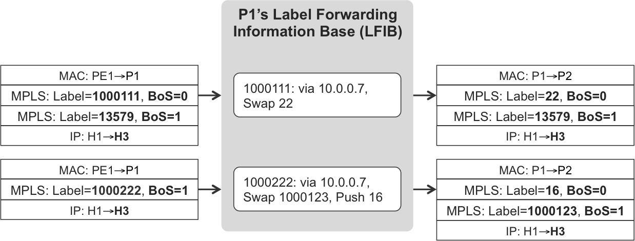
Figure 1-10. Other MPLS operations
MPLS Configuration and Forwarding Plane
MPLS interface configuration
The first step is to enable MPLS on the interfaces on which you want to forward MPLS packets. Example 1-7 shows the Junos configuration of one interface at PE1.
Example 1-7. MPLS interface configuration—PE1 (Junos)
1     interfaces {
2         ge-2/0/4 {
3              unit 0 {
4                 family mpls;
5     }}}
6     protocols {
7         mpls {
8             interface ge-2/0/4.0;
9     }}
Lines 1 through 4 enable the MPLS encapsulation on the interface, and lines 6 through 8 enable the interface for MPLS protocols. Strictly speaking, the latter configuration block is not always needed, but it is a good practice to systematically add it.
Note
Throughout this book, it is assumed that every MPLS-enabled interface in Junos has at least the configuration from Example 1-7.
In IOS XR, there is no generic MPLS configuration. You need to enable the interface for each of the MPLS flavors that you need to use. This chapter features the simplest of all the MPLS flavors: static MPLS. Example 1-8 presents the configuration of one interface at PE4.
Example 1-8. MPLS interface configuration—PE4 (IOS XR)
mpls static
 interface GigabitEthernet0/0/0/0
!
Label-switched path PE1→PE4—configuration
Remember that H1→H3 packets go through PE1 and PE4. You need an LSP that takes these packets from PE1 to PE4. Let’s make the LSP follow the path PE1-P1-P2-PE4 that we saw in Figure 1-9.
Note
This example is based on static LSPs, which are not scalable because they require manual label assignments at each hop of the path. Beginning in Chapter 2, the focus is on the much more scalable dynamic LSPs.
Example 1-9 gives the full configuration along the path.
Example 1-9. LSP PE1→PE4 configuration—Junos and IOS XR
#PE1 (Junos)

protocols {
    mpls {
        static-label-switched-path PE1--->PE4 {
            ingress {
                next-hop 10.0.0.3;
                to 172.16.0.44;
                push 1000001;
}}}}

#P1 (Junos)

protocols {
    mpls {
        icmp-tunneling;
        static-label-switched-path PE1--->PE4 {
            transit 1000001 {
                next-hop 10.0.0.7;
                swap 1000002;
}}}}

#P2 (IOS XR)

mpls static
 address-family ipv4 unicast
  local-label 1000002 allocate
   forward
    path 1 nexthop GigabitEthernet0/0/0/5 10.0.0.11 out-label pop
!
PE4 receives plain IPv4 packets from P2, so it does not require any LSP-specific configuration.
Labels 1000001 and 1000002 are locally significant to P1 and P2, respectively. Their numerical values could have been identical and they would still correspond to different instructions because they are not interpreted by the same LSR.
LSP PE1→PE4—forwarding plane
It’s time to inspect the forwarding instructions that steer the H1→H3 IPv4 packet through the PE1→PE4 LSP. Let’s begin at PE1, which is shown in Example 1-10.
Example 1-10. Routing and forwarding state at the ingress PE—PE1 (Junos)
1     juniper@PE1> show route receive-protocol bgp 172.16.0.201
2                  10.2.34.30 active-path
3
4     inet.0: 36 destinations, 45 routes (36 active, ...)
5       Prefix         Nexthop        MED     Lclpref    AS path
6     * 10.2.34.0/24   172.16.0.44    100     100        65002 I
7
8     juniper@PE1> show route 172.16.0.44
9
10    inet.0: 36 destinations, 45 routes (36 active, ...)
11    + = Active Route, - = Last Active, * = Both
12
13    172.16.0.44/32     *[IS-IS/18] 1d 11:22:00, metric 30
14                        > to 10.0.0.3 via ge-2/0/4.0
15
16    inet.3: 1 destinations, 1 routes (1 active, ...)
17    + = Active Route, - = Last Active, * = Both
18
19    172.16.0.44/32     *[MPLS/6/1] 05:00:00, metric 0
20                        > to 10.0.0.3 via ge-2/0/4.0, Push 1000001
21
22    juniper@PE1> show route 10.2.34.30 active-path
23
24    inet.0: 36 destinations, 45 routes (36 active...)
25    + = Active Route, - = Last Active, * = Both
26
27    10.2.34.0/24   *[BGP/170] 06:37:28, MED 100, localpref 100,
28                              from 172.16.0.201, AS path: 65002 I
29                    > to 10.0.0.3 via ge-2/0/4.0, Push 1000001
30
31    juniper@PE1> show route forwarding-table destination 10.2.34.30
32    Routing table: default.inet
33    Internet:
34    Destination   Next hop              Type  Index   NhRef Netif
35    10.2.34.0/24                        indr  1048575     3
36                  10.0.0.3 Push 1000001           513     2 ge-2/0/4.0
37
38    juniper@PE1> show mpls static-lsp statistics name PE1--->PE4
39    Ingress LSPs:
40    LSPname      To            State   Packets      Bytes
41    PE1--->PE4   172.16.0.44   Up        27694    2768320
The best BGP route to the destination 10.2.34.30 (H3) has a BGP next-hop attribute (line 6) equal to 172.16.0.44. There are two routes toward 172.16.0.44 (PE4’s loopback):
-
An IS-IS route in the global IPv4 routing table
inet.0(lines 10 through 14). -
A MPLS route in the
inet.3auxiliary table (lines 16 through 20). The static LSP configured in Example 1-9 automatically installs this MPLS route.
The goal of the inet.3 auxiliary table is to resolve BGP next hops (line 6) into forwarding next hops (line 20). Indeed, the BGP route 10.2.34.0/24 is installed in inet.0 with a labeled forwarding next hop (line 29) that is copied from inet.3 (line 20). Finally, the BGP route is installed in the forwarding table (lines 31 through 36) and pushed to the forwarding engines.
The fact that Junos has an auxiliary table (inet.3) to resolve BGP next hops is quite relevant. Keep in mind that Junos uses inet.0 and not inet.3 to program the forwarding table. For this reason, PE1’s default behavior is not to push any labels on the packets that it sends to internal (non-BGP) destinations such as PE4’s loopback, as demonstrated in Example 1-11.
Example 1-11. Unlabeled traceroute to a non-BGP destination—PE1 (Junos)
juniper@PE1> traceroute 172.16.0.44
traceroute to 172.16.0.44
 1  P1 (10.0.0.3)  42.820 ms  11.081 ms  4.016 ms
 2  P2 (10.0.0.25)  6.440 ms P2 (10.0.0.7)  3.426 ms *
 3  PE4 (10.0.0.11)  9.139 ms *  78.770 ms
Let’s get back to the PE1→PE4 LSP and move on to P1, the first LSR on the path.
Example 1-12. Routing and forwarding state at a transit P—P1 (Junos)
juniper@P1> show route table mpls.0 label 1000001

mpls.0: 5 destinations, 5 routes (5 active, 0 holddown, 0 hidden)
+ = Active Route, - = Last Active, * = Both

1000001    *[MPLS/6] 07:23:19, metric 1
            > to 10.0.0.7 via ge-2/0/3.0, Swap 1000002
The mpls.0 table stores label instructions. For example, if P1 receives a packet with label 1000001, the instruction says: swap the label for 1000002 and send the packet out of ge-2/0/3 to P2. This instruction set is known as the Label Forwarding Information Base (LFIB). The mpls.0 table is not auxiliary: it populates the forwarding table.
Finally, let’s look at P2’s LFIB in Example 1-13.
Example 1-13. Routing and forwarding state at a transit P—P2 (IOS XR)
RP/0/0/CPU0:P2#show mpls forwarding labels 1000002
Local  Outgoing    Outgoing     Next Hop        Bytes
Label  Label       Interface                    Switched
------ ----------- ------------ --------------- ------------
1000002 Pop         Gi0/0/0/5    10.0.0.11       8212650
There is no point in looking at PE4, which behaves like a pure IP router with respect to the H1→H3 packets.
LSP PE4→PE2—Configuration
For completeness, Example 1-14 presents the full configuration of the PE4→PE2 LSP.
Example 1-14. LSP PE4→PE2 configuration—IOS XR
#PE4 (IOS XR)
mpls static
 address-family ipv4 unicast
  local-label 1000200 allocate per-prefix 172.16.0.22/32
   forward
    path 1 nexthop GigabitEthernet0/0/0/0 10.0.0.10 out-label 1000110
!

#P2 (IOS XR)
mpls static
 address-family ipv4 unicast
  local-label 1000110 allocate
   forward
    path 1 nexthop GigabitEthernet0/0/0/0 10.0.0.4 out-label pop
!
The key syntax at PE4 is per-prefix: this says that in order to place a packet on an LSP whose tail end is PE2 (172.16.0.22), push label 1000110 and send it to P2.
The first label value (1000200) from Example 1-14 is not really part of the PE4→PE2 LSP. It means that if it receives an MPLS packet with the outermost label 1000200, PE4 puts the packet on the PE4→PE2 LSP by swapping the label for 1000110. This logic is not very relevant to the current example, where H3→H1 packets arrive unlabeled to PE4.
Example 1-15 demonstrates the routing and forwarding state at the ingress PE (PE4).
Example 1-15. Routing and forwarding state at the ingress PE—PE4 (IOS XR)
RP/0/0/CPU0:PE4#show bgp 10.1.12.0/24 brief
[...]
   Network        Next Hop       Metric LocPrf Weight Path
* i10.1.12.0/24   172.16.0.11       100    100      0 65001 i
*>i               172.16.0.22       100    100      0 65001 i

RP/0/0/CPU0:PE4#show cef 10.1.12.10
[...]
 local adjacency 10.0.0.10
   via 172.16.0.22, 2 dependencies, recursive [flags 0x6000]
    path-idx 0 NHID 0x0 [0xa137dd74 0x0]
    next hop 172.16.0.22 via 172.16.0.22/32

RP/0/0/CPU0:PE4#show cef 172.16.0.22
[...]
 local adjacency 10.0.0.10
   via 10.0.0.10, GigabitEthernet0/0/0/0, 4 dependencies, [...]
    next hop 10.0.0.10
    local adjacency
     local label 1000200      labels imposed {1000110}

RP/0/0/CPU0:PE4#show mpls forwarding labels 1000200
Local  Outgoing Prefix         Outgoing   Next Hop  Bytes
Label  Label    or ID          Interface            Switched
------ -------- -------------- ---------- --------- --------
1000200 1000110 172.16.0.22/32 Gi0/0/0/0  10.0.0.10 10410052
The logic in IOS XR is very similar, except that in this case there are no auxiliary tables. As a result, PE4’s default behavior is to push labels on the packets that it sends to internal (non-BGP) destinations that are more than a hop away, like PE2’s loopback shown in Example 1-16.
Example 1-16. Labeled traceroute to a non-BGP destination—PE4 (IOS XR)
RP/0/0/CPU0:PE4#traceroute 172.16.0.22

 1  p2 (10.0.0.10) [MPLS: Label 1000110 Exp 0] 9 msec ...
 2  pe2 (10.0.0.4) 0 msec ...
End-to-end user traffic
After the PE1→PE4 and the PE4→PE2 LSPs are up, end-to-end connectivity is fine.
Example 1-17. End-to-end user traceroute through an MPLS network
RP/0/0/CPU0:H1#traceroute vrf H1 10.2.34.30

 1  ce1 (10.1.12.1) 0 msec ...
 2  pe1 (10.1.0.1) 0 msec ...
 3  p1 (10.0.0.3) [MPLS: Label 1000001 Exp 0] 9 msec ...
 4  p2 (10.0.0.7) [MPLS: Label 1000002 Exp 0] 9 msec ...
 5  pe4 (10.0.0.11) 9 msec ...
 6  br4 (10.2.0.4) 9 msec ...
 7  h3 (10.2.34.30) 9 msec ...
As expected, traceroute shows the forward path with the PE1→PE4 LSP’s labels.
You might wonder how P1 can send an Internet Control Message Protocol (ICMP) Time Exceeded message to H1, taking into account that it does not even have a route to reach H1. What happens is the following:
-
P1 receives a UDP packet with MPLS label 1000001 and MPLS TTL =1.
-
P1 decrements the TTL, detects that it expired, and encapsulates the original UDP packet with MPLS label 1000001 inside an ICMP Time Exceeded packet, which is in turn encapsulated with MPLS label 1000002. This packet has TTL=255.
-
P1 sends the MPLS-encapsulated ICMP Time Exceeded packet to P2, which pops the label and sends the packet to PE4.
-
PE4 looks at the destination of the ICMP Time Exceeded packet, which is H1. According to a regular IPv4 lookup, PE4 sends this packet through the PE4→PE2 LSP, and this is how it gets to H1.
Tip
This mechanism works by default in IOS XR, but you must explicitly activate it in Junos by using the command set protocols mpls icmp-tunneling.
Forwarding Equivalence Class
The previous example focused on the communication between two hosts, H1 and H3. Let’s take one step back and think of the global Internet. Imagine that PE1 chooses PE4 as the BGP next hop for 100,000 routes. Think twice: all of these 100,000 routes have the same BGP next hop. This means that PE1 can send all the packets toward any of these 100,000 prefixes through the same LSP. Of course, this can raise concerns with regard to load balancing and redundancy, but these topics are fully covered in this book.
Every packet that PE1 maps to the PE1→PE4 LSP belongs to a single Forwarding Equivalence Class (FEC). The transit LSRs only need to know how to forward in the context of this FEC: basically, just one entry in the LFIB. Thus, trillions of flows can be successfully forwarded with just one forwarding entry.
Note
Forwarding state aggregation is one of the first immediate benefits of MPLS.
Again, What Is MPLS?
MPLS is not an encapsulation. It is an architectural framework that decouples transport from services. In this case, the service is Internet access (IPv4 unicast) and the transport is performed by MPLS LSPs.
This decoupling is achieved by encoding instructions in packet headers. Whether the encapsulation is MPLS or something else, the MPLS paradigm remains.
The Internet is living proof of how MPLS is a cornerstone of network service scalability. Every second that our user, Annika, is in a video conference with her friend Ruijiao, more than 1,000 MPLS labels are pushed, swapped, or popped to make it happen. The core devices that do these label operations have no visibility of the public IP addresses that Annika’s and Ruijiao’s terminals use to connect to the Internet.
Another important aspect of MPLS is instruction stacking. Whether these instructions are in the form of labels or something else, being able to stack them is equivalent to providing a sequence of instructions. For network services that go beyond simple connectivity, this is a key enabler.
As discussed later in Chapter 10, scalable network architectures have a North-South and an East-West direction. Instruction stacking introduces another dimension: Up-Down.
Note
MPLS is a natural fit for architectures with a feature-rich network edge combined with a fast and resilient backbone.
MPLS was born for the Internet. It started small and continues to grow. The initial goal of MPLS was to solve a very specific challenge, but now it keeps evolving to meet many other requirements in terms of service, transport, class of service, performance, resilience, and so on.
OpenFlow
The SDN era started with an experimental protocol that created a high level of expectation: OpenFlow.
OpenFlow enables flow-based programmability of a forwarding engine. Its initial version (v1.0) is basically a network switch abstraction. Over time, different versions of OpenFlow have incorporated more functionality, the details of which are beyond the scope of this book. You can find all the definitions and specifications at the Open Networking Forum (https://www.opennetworking.org/sdn-resources/openflow).
Figure 1-11 shows OpenFlow v1.0 at work. OpenFlow assumes that there is a central controller software running as a virtual machine (VM), or as a container, or directly on the host OS of a server. The controller must have IP connectivity to the switches by using either of the following:
-
An out-of-band network that is not under the command of the controller
-
An in-band network connection that relies on some preexisting forwarding state
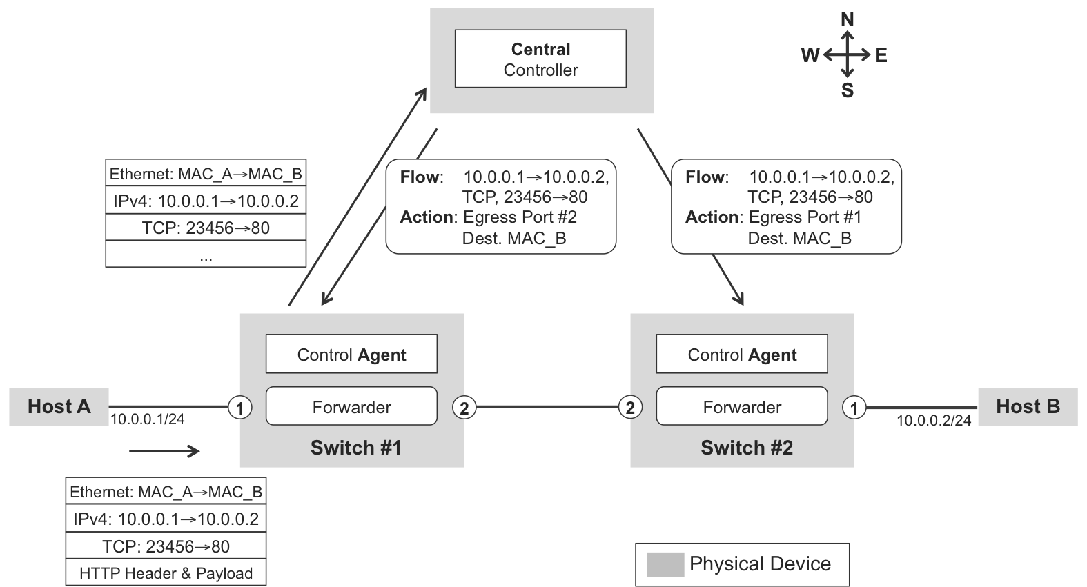
Figure 1-11. Openflow in action
Switches have a lightweight control plane and a comparatively more powerful forwarding engine. The most important piece of state on an OpenFlow-controlled switch is its flow table. The switches’ control plane is connected to the central controller via an OpenFlow TCP session, whose purpose is to exchange OpenFlow messages.
Figure 1-11 shows Host A sending the first packet of a user TCP flow to Host B. When the packet arrives to port 1, Switch #1 realizes that this flow is not programmed on its flow table, so its control agent “punts” the packet to the controller. The controller had previously learned where Host B is, and with this information it is able to program the new flow on the switches. At this point, the switches are able to forward this flow’s packets to the destination.
OpenFlow—Flow-Based Forwarding
One fundamental architectural attribute of OpenFlow is its per-flow programmability, offering a fine granularity when it comes to defining flows and their associated actions. This results in a flow-based forwarding model. For decades, the industry has produced a wide variety of both flow-based forwarding and packet-based forwarding solutions. Which model is better? Neither—both are. It really depends on the use case.
There are parts of the network where even thinking about flow-based forwarding is out of the question, like in the core and most of the broadband edge functions, because it would not scale and there is no need for it. The Internet requires state aggregation (FECs) instead of state expansion (flows). Keeping state for flows is inherently more expensive and complex than doing packet-based forwarding. However, there are other network functions, such as firewalling, DPI, and CGNAT, among others, that need to be flow-based due to the nature of the function they execute.
The same principles by which the industry has naturally selected which parts of the network should be flow-based and which should not are still completely valid. The fact that there is a new protocol to program flows on a network does not make flow-based forwarding either a better or worse idea.
New developments in forwarding technology, memory, and costs, could shift things in one direction or the other. For this reason, it is wise to decouple the existence of the OpenFlow protocol from the debate of whether flow-based forwarding is a good idea or not. In fact, OpenFlow, as such, does not mandate nor specify the granularity of the flows to be programmed.
When deciding to use one model or the other, the first question to answer is do you need flow-based forwarding? If not, it’s better to use packet-based forwarding. Data center fabrics (described in Chapter 10) are a good example of the risks involved in blindly moving to a flow-based forwarding paradigm. At first glance, it looks like a good fit, but a deeper analysis proves that it really depends on the primary use of the data center.
Ivan Pepelnjak wrote an enlightening article called “OpenFlow and Fermi Estimates,” which is included in his book, SDN and OpenFlow—The Hype and the Harsh Reality (self-published, 2014, http://www.ipspace.net/Books). You might have realized that your web browser automatically establishes connections to many URLs that you had no intention to visit. For example, when you read your favorite online newspaper, a wide variety of content—such as advertisements, multimedia, and stats—are automatically loaded from external sites. Every piece of content is retrieved via an individual short-lived connection. It is this short-lived characteristic of many Internet flows that makes flow programming a very intensive task. This is particularly true for high-speed data center switches, which have a comparatively weak control plane. Pepelnjak’s Fermi estimate shows that the forwarding capacity of a typical data center switch is reduced by several orders of magnitude when it must perform flow-based forwarding of HTTP flows. The control plane becomes the bottleneck in this case, so most of the bandwidth cannot be used. If your network transports short-lived flows, use OpenFlow carefully.
OpenFlow—Openness and P4
OpenFlow is an open protocol and P4 (a newer high-level language—programming protocol-independent packet processors—thus four Ps) takes it one step further, from a protocol to a programming language. Despite the definitions, not everyone agrees on whether OpenFlow and P4 are actually high level or low level.
No wonder, openness is cool. On the other hand, implementing fine-grained edge features is complex. There is no way around it. Regardless of whether the complexity is on the application-specific integrated circuits (ASICs), or on the low-level microcode, or on high-level instructions, it must be somewhere, and not every approach is equally efficient or flexible. Standardizing a high-level language hides complexity, which is great, but for many features, developers need to go down to the lower levels.
There is value in low-level languages because they provide flexibility due to how close they are to the actual hardware. They are, and must be, inherently specific, and if they want to be generic, they will precisely lose that specificity. Hardware has differences that must be exposed because there is a lot of innovation that vendors are adding to their ASICs to differentiate them from one another. If they are exposed, the language becomes specific. If they are not exposed, the innovation is lost, and the system becomes a disincentive to innovation.
At a certain low level, the relationship between hardware and the software that programs it is very intimate. Trying to insert a layer between, even an industry-defined layer, is not guaranteed to boost innovation. Only time will tell whether standardizing the way that a network device is programmed brings innovation or slows down the new feature implementations. It will certainly be an interesting story to watch or in which to at least play a role.
Another important characteristic of the OpenFlow model is the decoupling of the control and forwarding planes. Let’s discuss this topic in the broader context of SDN.
SDN
This book does not attempt to redefine the SDN concept itself: this is up to the inventors of the acronym. What this book takes the liberty of describing is the SDN era. Let’s first discuss the official definition of SDN and then later move on to the SDN era.
SDN has been defined by Open Networking Forum (https://www.opennetworking.org) as follows:
The physical separation of the network control plane from the forwarding plane, and where a control plane controls several devices.
Following this definition, it states:
Software-Defined Networking (SDN) is an emerging architecture that is dynamic, manageable, cost-effective, and adaptable, making it ideal for the high-bandwidth, dynamic nature of today’s applications. This architecture decouples the network control and forwarding functions enabling the network control to become directly programmable and the underlying infrastructure to be abstracted for applications and network services. The OpenFlow™ protocol is a foundational element for building SDN solutions.
Separation of the Control and Forwarding Planes
The process of decoupling the control and the forwarding planes is presented as a key element that drives SDN adoption; however, some engineers contend that such separation has existed for many years on their own networks. For example, both Juniper and Cisco routers clearly separated the control and forwarding planes in the 1990s. The fact that they were running on the same physical chassis did not negate such separation, which was, in fact, fundamental to enable growth on the Internet. When Juniper introduced such separation, along with ASIC-based forwarding, it triggered an era of unprecedented capacity growth. And with hindsight, it was required to sustain the unprecedented traffic growth that lay ahead.
Since the early 2000s—a few years before OpenFlow was proposed—networking vendors have implemented and shipped solutions that instantiate the control plane on an external physical device. This is essentially a controller that programs the so-called “line card chassis.”
It is therefore fair to note that the fundamental architectural attribute associated with SDN, separating the control and forwarding planes, is not essentially new, and is widely used already on the networks. Anyway, new or not, this attribute is valuable.
Another fundamental architectural ingredient of SDN is centralization. Sometimes it is logical centralization, because physical centralization is not always feasible. If you assume that the control plane of your network is physically decoupled from the forwarding plane, it leads to an interesting set of challenges:
-
You need a network to connect both functions (the control and forwarding planes). If such a network fails, how does the solution work?
-
There are latency constraints for proper interworking between the control and forwarding planes. Latency is important for resiliency, response to network events, telemetry, and so on. How far can the controller be from the forwarding elements?
It is not trivial to generalize, for any network, a way that these principles can be applied. SDN’s principles are better analyzed in the context of specific use cases. You can then see if an architecture that adheres to these principles is feasible or not.
Separating the control and forwarding planes—data center overlays
A paradigmatic use case for which SDN principles fit well is the overlay architecture at data centers, assuming the following:
-
There is an underlay fabric that provides resilient connectivity between the overlay’s forwarding plane (usually a vRouter or a vSwitch on a server) and the control plane (central controller).
-
The latency is contained within specific working limits.
Separating the control and forwarding planes—WAN IP/MPLS
Let’s now analyze the applicability of the SDN architectural principles to the WAN IP/MPLS network on any ISP. Although there are certain control plane functions that we can centralize, it is unfeasible to achieve a full centralization. Indeed, if you place the entire control plane hundreds or thousands of kilometers (and N network hops) away from the forwarding plane, it is not possible to guarantee the interaction between both planes in a reliable and responsive way. For this reason, the SDN concept can only be applied to the WAN environment in a tactical manner.
Having some centralized network-wide control intelligence can lead to more accurate calculations, which is very useful for cases such as Traffic Engineering. In this case, the distributed control plane is enhanced by an additional centralized intelligence. This is fully explained in Chapter 15.
These examples show that SDN can have different levels of applicability for each scenario (no one-size-fits-all). Network vendors have applied this design principle over the years to many technology and architecture designs: centralize what you can, distribute what you must. If something can be centralized, and there are no physical or functional constraints, centralize it; otherwise, it should be left distributed.
SDN and the Protocols
It is fair to claim that OpenFlow was a spark that caused a mind shift in the industry, triggering a healthy debate that has acted as a catalyzer for the SDN era.
That having been said, there is some controversy about the technical relevance of OpenFlow. Whereas some engineers believe that OpenFlow is the cornerstone of SDN, others believe that it does not propose anything fundamentally new. In all fairness, as with any other protocol or technology, OpenFlow is evolving through its different versions. Whether it will really enable a fundamental benefit in the future or not, only time will tell.
In parallel with the continual development of OpenFlow, other industry forums such as IETF have also been developing similar concepts. In fact, two of the IETF’s crown jewels, BGP and MPLS, are gaining momentum as SDN-enabler protocols.
It is not surprising to find BGP in the SDN era, because it is the most scalable networking protocol that ever has been designed and implemented. On the other hand, the MPLS paradigm (decoupling service from transport, placing instructions on packet headers) is gaining an ever-growing relevance in the development and deployment of scalable SDN solutions. This paradigm has indeed been renamed by the OpenFlow community as SDN 2.0.
Note
Remember that the MPLS paradigm is not an encapsulation.
Chapter 11 and Chapter 12 describe production-ready SDN solutions mainly based on BGP—and its derivatives—in combination with the MPLS paradigm.
In practice, OpenFlow is an optional element of the SDN-like architectures. Many modern SDN-like solutions do not rely on OpenFlow and are not even inspired by it. Others do: of course, OpenFlow belongs to the SDN era.
Some parallel IETF projects concentrate on standardizing the way to program and configure the network elements’ behavior (e.g., PCEP, BGP Flowspec, NETCONF/YANG/OpenConfig, I2RS, and ForCES). Although some have not been widely adopted, others are gaining momentum and they also belong to the SDN era. Chapter 15 covers PCEP in detail.
Regardless of the terminology debate and the protocol choice, one thing is certain: the industry will continue exploring and implementing new architectures that are certainly changing the way we see and use networking.
The SDN Era
If you look at all the SDN-like implementations and technologies, you’ll find two elements in common that reveal what was missing at the beginning of the century in our industry:
- Automation
- Creating the conditions to automate actions on the networks (configuration, provisioning, operation, troubleshooting, etc.)
- Abstraction
- Achieving North-South communication by surpassing the vendor-specific barriers and complexities that customers had to adapt to, or avoid
If you look at how the industry has adopted two protocols such as OpenFlow or Netconf, the focus has typically been on the “how”: how to program low-level flows or how to configure a device. However, what the industry really needs is a focus on the “what”: what is the intent. It is going high level, going abstract, which enables defining intents and automating actions around those intents. In other words: “Say what you want, not how you want it.” Then make the network intelligent enough to decide the best “how” possible.
In summary, what is common across the myriad SDN terms and cross initiatives, industry wide, is automation and abstraction. This is the real essence of what this book considers the SDN era and that we, as an industry, should probably care about. Let’s briefly look at a few specific use cases of new technologies that seem to provide concrete added value to real customer challenges through automation and abstraction.
SDN-Era Use Cases
If we step away from the term SDN and its many interpretations, there are in fact new solutions and technologies developed for specific use cases that involve both an architectural change, and a response to a real problem. The following is a list of representative scenarios that are part of the new thinking in the SDN era. Some use tested technologies in a practical, often brilliant, way.
Data center
The data center requirements have grown by orders of magnitude in many dimensions, and very rapidly. Data centers have suffered a rapid transition from being mere dense LANs into hyperscale infrastructures with very strict requirements not only in performance but also in latency, scale, multitenancy, and security. And associated with all of that is the need for improved manageability.
Some proposed data center switching infrastructures are based on OpenFlow with a central controller programming flows along the path, but the industry has also looked at other architectures and technologies that have proven to deliver on the same requirements at scale. You do not need to look far to find them: the Internet itself. The suite of protocols and architectures used to build the Internet and the ISP IP networks have become the best mirror to look at to build the next generation data centers that do the following:
-
Decouple transport from services (the architectural principle of MPLS)
-
Build a stable, service-agnostic transport infrastructure (fabrics)
-
Provision services only at the edge, and use scalable protocols for the control plane (BGP)
This ISP architecture has been adapted to data centers in several ways. First, the underlay’s forwarding plane is optimized to the specific requirements of data centers, which include very low latency among the end systems (servers) and very high transport capacity with almost no restriction.
The ISP’s edge is replaced with the data center’s overlay-capable edge forwarders, typically instantiated by the vRouter/vSwitch on server hypervisors or eventually the Top-of-Rack (ToR) switch.
This provides a good opportunity to use a central controller that is capable of programming the edge forwarders as if they were the packet forwarding engines or the line cards of a multicomponent physical network device. You can see this model in detail throughout Chapter 11.
WAN
The ISP WAN—the internal ISP backbone—is another specific use case for which there are new challenges that need to be addressed. Bandwidth resources are scarcer than ever, and CAPEX control levels make it impossible to deploy as much capacity as in the past. However, traffic continues to grow, and a growing variety of services flow across the WAN infrastructure, raising the need for mechanisms that are capable of managing these resources more efficiently and dynamically. MPLS Traffic Engineering has existed for many years, but the distributed nature of the Traffic Engineering decisions led to inefficiencies.
Now, with the broader availability and implementations of protocols such as PCEP, it is possible to enable centralized intelligent controllers that complement the distributed control plane of the network, by adding a network-wide vision and decision process. The ISP WAN can now take advantage of implementations that offer intelligent management of resources and automation for tasks that previously could only be done in a limited fashion and to some extent manually, or were simply not done, because there was enough capacity. The resource scarcity and the business requirements now mandate a different way of doing it, and this is another example and use case of new implementations that employ long-standing concepts, such as the PCE Client-Server architecture. This model is detailed in Chapter 15.
Packet-optical convergence
Packet-based and circuit-based switching are two fundamentally different paradigms, and they both have reasons to exist. Traditionally they have been separate layers, most of the time with the circuit-switching network as the server layer for the packet-switching network (the client). This role is sometimes reversed; for example—with TDM emulated circuits over MPLS in Mobile backhaul scenarios, briefly discussed in Chapter 6.
Optical networks are the most common circuit-switched technology. They provide optical circuits that packet-based networks use for point-to-point communication among the different packet-switching nodes (routers, switches, etc.).
In the SDN era, the vast majority of the traffic is becoming IP—even mobile voice with technologies such as VoLTE. It is already a fact that the main (if not only) purpose of the optical network is to transport the IP network. For this reason, the tight coordination and optimization of the optical and IP networks becomes business critical. Any inefficiency on such integration immediately becomes a large source of extra CAPEX and OPEX.
Therefore, here’s another area where ISPs face a strong challenge that requires specific solutions. The need for resource coordination, automation, and optimization is addressed by doing the following:
-
Exposing resources in a normalized way (abstraction)
-
Having the ability to automate the right resource allocation decisions (set up paths, optimize paths, search for backup resources, etc.) while considering both the optical layer and the packet layer
Again, the role of a centralized controller is paramount. The model described in Chapter 15 is also targeting this use case.
IP peering
IP peering provides another opportunity to enhance and optimize the existing mechanisms. So far, the IP peering points’ behavior has been exclusively governed by BGP protocol rules. BGP implements a decision algorithm that searches for the best loop-free path—loop-free in the sense that the AS path does not contain the same AS twice. Although many tools such as BGP attributes can be used to influence the decision process, it still remains a built-in algorithm that is based on certain predefined rules. Such rules may not take into account business-related aspects that a provider could need to consider in order to make the best routing decisions.
Some of these business aspects are the price of the peering connection (it might be a transit link), the actual latency to the destination (shorter AS paths do not necessarily imply lower latency), link occupation, and maybe others. As business conditions become stricter in our industry, network decisions need to factor in more variables.
ISPs often use ad hoc tunneling overlays (based on IP or MPLS) to bypass the default forwarding decisions, but this approach does not scale: ISPs deserve a better solution.
A controller-based solution that addresses this opportunity needs to have detailed visibility of all the BGP routing state in the SP. The BGP Monitoring Protocol (BMP), implemented in both Junos and IOS XR, accommodates retrieving from a given router:
- The Adj-RIB-in
- These are the prefixes that the polled router has received from a peer, prior to the application of import routing policies.
- The Adj-RIB-out
- These are the prefixes that the polled router has advertised to a peer, after the application of export routing policies.
Additionally, enhanced telemetry mechanisms are being implemented to retrieve significant traffic statistics. Putting all together, such a solution is definitely feasible in the mid-term future.
This is another example of a real customer challenge that can be solved in the SDN era by a partial centralization of the decision process through incremental intelligence. And it’s another case of automation and abstraction.
The branch office
The services offered at the branch office have been substantially static. SPs are looking at ways to offer more dynamic services that the customer might even self-provision. These services can reduce operating expenses by delegating some tasks to the customer, and at the same time help increase the revenue through a faster service adoption (point-and-click customer service-provisioning) and new business models (try-and-buy).
This is an old aspiration from SPs and has been the object of traditional technologies such as policy servers, PCRF, Radius/CoA, and the like. For example, the so-called Turbo Button, with which the customer can increase the bandwidth temporarily of its broadband connection, or the self-provisioning portals that enable it, among other possibilities, have existed in the industry for many years. However, the market and business is now rising and more SPs are interested in actively offering these options.
Today, in the SDN era, the business pressure threatens sustainability, so increasing top-line revenue becomes a must through offering more flexible services. This is an opportunity for new emerging solutions based on centralized controllers that implement flexible and automated services configuration.
Although these scenarios use existing technologies and do not represent any radical architectural shift, all of these use cases represent a clever combination of one or more of the following attributes:
-
Automation and abstraction
-
Complementing the intelligence of the existing infrastructure
-
Making the network decisions more dynamic
-
Decoupling overlay from underlay in order to scale
These attributes are what the authors intend to apply to the book’s many chapters on MPLS, making it fundamentally a key tool in the SDN era.
Get MPLS in the SDN Era now with the O’Reilly learning platform.
O’Reilly members experience books, live events, courses curated by job role, and more from O’Reilly and nearly 200 top publishers.

