Chapter 4. Data Structures
In previous chapters, we examined some distinctions between the different components that make up an Oracle database. For example, you’ve learned that the Oracle instance differs from the files that make up the physical storage of the data in tablespaces, that you cannot access the data in a tablespace except through an Oracle instance, and that the instance itself isn’t very valuable without the data stored in those files.
In the same way, the actual tables and columns within the database are the entities stored within the database files and accessed through the database instance. The user who makes a request for data from an Oracle database probably doesn’t know anything about instances and tablespaces, but does know about the structure of her data, as implemented with tables and columns. To fully leverage the power of Oracle, you must understand how the Oracle database server implements and uses these logical data structures.
Datatypes
The datatype is one of the attributes for a column or a variable in a stored procedure. A datatype describes and limits the type of information stored in a column, and limits the operations that you can perform on columns.
You can divide Oracle datatype support into three basic varieties: character datatypes, numeric datatypes, and datatypes that represent other kinds of data. You can use any of these datatypes when you create columns in a table, as with this SQL statement:
CREATE SAMPLE_TABLE(
        char_field CHAR(10),
        varchar_field VARCHAR2(10),
        todays_date DATE)
You also use these datatypes when you define variables as part of a PL/SQL procedure.
Character Datatypes
Character datatypes can store any string value, including the string representations of numeric values. Assigning a value larger than the length specified or allowed for a character datatype results in a runtime error. You can use string functions, such as UPPER, LOWER, SUBSTR, and SOUNDEX, on standard (not large) character value types.
There are several different character datatypes:
- CHAR
The CHAR datatype stores character values with a fixed length. A CHAR datatype can have between 1 and 2,000 characters. If you don’t explicitly specify a length for a CHAR, it assumes the default length of 1. If you assign a value that’s shorter than the length specified for the CHAR datatype, Oracle will automatically pad the value with blanks. Some examples of CHAR values are:
CHAR(10) = "Rick ", "Jon ", "Stackowiak"
- VARCHAR2
The VARCHAR2 datatype stores variable-length character strings. Although you must assign a length to a VARCHAR2 datatype, this length is the maximum length for a value rather than the required length. Values assigned to a VARCHAR2 datatype aren’t padded with blanks. The VARCHAR2 datatype can have up to 4,000 characters. Because of this, a VARCHAR2 datatype can require less storage space than a CHAR datatype, because the VARCHAR2 datatype stores only the characters assigned to the column.
At this time, the VARCHAR and VARCHAR2 datatypes are synonymous in Oracle8 and later versions, but Oracle recommends the use of VARCHAR2 because future changes may cause VARCHAR and VARCHAR2 to diverge. The values shown earlier for the CHAR values, if entered as VARCHAR2 values, are:
VARCHAR2(10) = "Rick", "Jon", "Stackowiak"
- NCHAR and NVARCHAR2
The NCHAR and NVARCHAR2 datatypes store fixed-length or variable-length character data using a different character set from the one used by the rest of the database. When you create a database, you specify the character set that will be used for encoding the various characters stored in the database. You can optionally specify a secondary character set as well (this is known as the National Language Set , or NLS). The secondary character set will be used for NCHAR and NVARCHAR2 columns. For example, you may have a description field in which you want to store Japanese characters while the rest of the database uses English encoding. You would specify a secondary character set that supports Japanese characters when you create the database, and then use the NCHAR or NVARCHAR2 datatype for the columns in question.
With Oracle9i, you can specify that you want to indicate the length of NCHAR and NVARCHAR2 columns in terms of characters, rather than bytes. This new feature allows you to indicate, for example, that a column with one of these datatypes is 7 characters long. The Oracle9i database will automatically make the conversion to 14 bytes of storage if the character set requires double byte storage.
Note
Oracle Database 10g includes the Globalization Development Kit (GDK), which is designed to aid in the creation of Internet applications that will be used with different languages. The key feature of this kit is a framework that implements best practices for globalization for Java and PL/SQL developers.
Oracle Database 10g also supports case- and accent-insensitive queries and sorts. You can use this feature if you want to use only base letters or only base letters and accents in a query or sort.
- LONG
The LONG datatype can hold up to 2 GB of character data. It is regarded as a legacy datatype from earlier versions of Oracle. If you want to store large amounts of character data, Oracle now recommends that you use the CLOB and NCLOB datatypes. There are many restrictions on the use of LONG datatypes in a table and within SQL statements, such as the fact that you cannot use LONGs in WHERE, GROUP BY, ORDER BY, or CONNECT BY clauses or in SQL statements with the DISTINCT qualifier. You also cannot create an index on a LONG column.
- CLOB and NCLOB
The CLOB and NCLOB datatypes can store up to 4 GB of character data prior to Oracle Database 10g. With Oracle Database 10g, the limit has been increased to 128 TBs, depending on the block size of the database. The NCLOB datatype stores the NLS data. Oracle Database 10g implicitly performs conversions between CLOBs and NCLOBs. For more information on CLOBs and NCLOBs, please refer to the discussion about large objects (LOBs) in “Other Datatypes,” later in this chapter.
Numeric Datatype
Oracle uses a standard, variable-length internal format for storing numbers. This internal format can maintain a precision of up to 38 digits.
The numeric datatype for Oracle is NUMBER. Declaring a column or variable as NUMBER will automatically provide a precision of 38 digits. The NUMBER datatype can also accept two qualifiers, as in:
column NUMBER( precision, scale )
The precision of the datatype is the total number of significant digits in the number. You can designate a precision for a number as any number of digits up to 38. If no value is declared for precision, Oracle will use a precision of 38. The scale represents the number of digits to the right of the decimal point. If no scale is specified, Oracle will use a scale of 0.
If you assign a negative number to the scale, Oracle will round the number up to the designated place to the left of the decimal point. For example, the following code snippet:
column_round NUMBER(10,-2)
column_round = 1,234,567
will give column_round a value of 1,234,600.
The NUMBER datatype is the only datatype that stores numeric values in Oracle. The ANSI datatypes of DECIMAL, NUMBER, INTEGER, INT, SMALLINT, FLOAT, DOUBLE PRECISION, and REAL are all stored in the NUMBER datatype. The language or product you’re using to access Oracle data may support these datatypes, but they’re all stored in a NUMBER datatype column.
Date Datatype
As with the NUMERIC datatype, Oracle stores all dates and times in a standard internal format. The standard Oracle date format for input takes the form of DD- MON-YY HH:MI:SS, where DD represents up to two digits for the day of the month, MON is a three-character abbreviation for the month, YY is a two-digit representation of the year, and HH, MI, and SS are two-digit representations of hours, minutes, and seconds, respectively. If you don’t specify any time values, their default values are all zeros in the internal storage.
You can change the format you use for inserting dates for an instance by changing the NLS_DATE_FORMAT parameter for the instance. You can do this for a session by using the ALTER SESSION SQL statement or for a specific value by using parameters with the TO_DATE expression in your SQL statement.
Oracle SQL supports date arithmetic in which integers represent days and fractions represent the fractional component represented by hours, minutes, and seconds. For example, adding .5 to a date value results in a date and time combination 12 hours later than the initial value. Some examples of date arithmetic are:
12-DEC-99 + 10 = 22-DEC-99
31-DEC-1999:23:59:59 + .25 = 1-JAN-2000:5:59:59
As of Oracle9i, Release 2, Oracle also supports two INTERVAL datatypes, INTERVAL YEAR TO MONTH and INTERVAL DAY TO SECOND, which are used for storing a specific amount of time. This data can be used for date arithmetic.
Other Datatypes
Aside from the basic character, number, and date datatypes, Oracle supports a number of specialized datatypes:
- RAW and LONG RAW
Normally, your Oracle database not only stores data but also interprets it. When data is requested or exported from the database, the Oracle database sometimes massages the requested data. For instance, when you dump the values from a NUMBER column, the values written to the dump file are the representations of the numbers, not the internally stored numbers.
The RAW and LONG RAW datatypes circumvent any interpretation on the part of the Oracle database. When you specify one of these datatypes, Oracle will store the data as the exact series of bits presented to it. The RAW datatypes typically store objects with their own internal format, such as bitmaps. A RAW datatype can hold 2 KB, while a LONG RAW datatype can hold 2 GB.
- ROWID
The ROWID is a special type of column known as a pseudocolumn. The ROWID pseudocolumn can be accessed just like a column in a SQL SELECT statement. There is a ROWID pseudocolumn for every row in an Oracle database. The ROWID represents the specific address of a particular row. The ROWID pseudocolumn is defined with a ROWID datatype.
The ROWID relates to a specific location on a disk drive. Because of this, the ROWID is the fastest way to retrieve an individual row. However, the ROWID for a row can change as the result of dumping and reloading the database. For this reason, we don’t recommend using the value for the ROWID pseudocolumn across transaction lines. For example, there is no reason to store a reference to the ROWID of a row once you’ve finished using the row in your current application.
You cannot set the value of the standard ROWID pseudocolumn with any SQL statement.
The format of the ROWID pseudocolumn changed with Oracle8. Beginning with Oracle8, the ROWID includes an identifier that points to the database object number in addition to the identifiers that point to the datafile, block, and row. You can parse the value returned from the ROWID pseudocolumn to understand the physical storage of rows in your Oracle database.
You can define a column or variable with a ROWID datatype, but Oracle doesn’t guarantee that any value placed in this column or variable is a valid ROWID.
- ORA_ROWSCN
Oracle Database 10g supports a new pseudocolumn, ORA_ROWSCN, which holds the System Change Number (SCN) of the last transaction that modified the row. You can use this pseudocolumn to check easily for changes in the row since a transaction started. For more information on SCNs, see the discussion of concurrency in Chapter 7.
- LOB
A LOB, or large object datatype, can store up to 4 GB of information. LOBs come in three varieties:
You can designate that a LOB should store its data within the Oracle database or that it should point to an external file that contains the data.
LOBs can participate in transactions. Selecting a LOB datatype from Oracle will return a pointer to the LOB. You must use either the DBMS_LOB PL/SQL built-in package or the OCI interface to actually manipulate the data in a LOB.
To facilitate the conversion of LONG datatypes to LOBs, Oracle9i includes support for LOBs in most functions that support LONGs, as well as a new option to the ALTER TABLE statement that allows the automatic migration of LONG datatypes to LOBs.
- BFILE
The BFILE datatype acts as a pointer to a file stored outside of the Oracle database. Because of this fact, columns or variables with BFILE datatypes don’t participate in transactions, and the data stored in these columns is available only for reading. The file size limitations of the underlying operating system limit the amount of data in a BFILE.
- XMLType
As part of its support for XML, Oracle9i includes a new datatype called XMLType. A column defined as this type of data will store an XML document in a character LOB column. There are built-in functions that allow you to extract individual nodes from the document, and you can also build indexes on any particular node in the XMLType document.
- User-defined data
Oracle8 and later versions allow users to define their own complex datatypes, which are created as combinations of the basic Oracle datatypes previously discussed. These versions of Oracle also allow users to create objects composed of both basic datatypes and user-defined datatypes. For more information about objects within Oracle, see Chapter 13.
- AnyType, AnyData, AnyDataSet
Oracle9i and newer releases include three new datatypes that can be used to explicitly define data structures that exist outside the realm of existing datatypes. Each of these datatypes must be defined with program units that let Oracle know how to process any specific implementation of these types.
Type Conversion
Oracle automatically converts some datatypes to other datatypes, depending on the SQL syntax in which the value occurs.
When you assign a character value to a numeric datatype, Oracle performs an implicit conversion of the ASCII value represented by the character string into a number. For instance, assigning a character value such as 10 to a NUMBER column results in an automatic data conversion.
If you attempt to assign an alphabetic value to a numeric datatype, you will end up with an unexpected (and invalid) numeric value, so you should make sure that you’re assigning values appropriately.
You can also perform explicit conversions on data, using a variety of conversion functions available with Oracle. Explicit data conversions are better to use if a conversion is anticipated, because they document the conversion and avoid the possibility of going unnoticed, as implicit conversions sometimes do.
Concatenation and Comparisons
The concatenation operator for Oracle SQL on most platforms is two vertical lines (||). Concatenation is performed with two character values. Oracle’s automatic type conversion allows you to seemingly concatenate two numeric values. If NUM1 is a numeric column with a value of 1, NUM2 is a numeric column with a value of 2, and NUM3 is a numeric column with a value of 3, the following expressions are TRUE:
NUM1 || NUM2 || NUM3 = "123"
NUM1 || NUM2 + NUM3 = "15" (12 + 3)
NUM1 + NUM2 || NUM3 = "33" (1+ 2 || 3)
The result for each of these expressions is a character string, but that character string can be automatically converted back to a numeric column for further calculations.
Comparisons between values of the same datatype work as you would expect. For example, a date that occurs later in time is larger than an earlier date, and 0 or any positive number is larger than any negative number. You can use relational operators to compare numeric values or date values. For character values, comparisons of single characters are based on the underlying code pages for the characters. For multicharacter strings, comparisons are made until the first character that differs between the two strings appears. The result of the comparison between these two characters is the result of the overall comparison.
If two character strings of different lengths are compared, Oracle uses two different types of comparison semantics: blank-padded comparisons and non-padded comparisons . For a blank-padded comparison, the shorter string is padded with blanks and the comparison operates as previously described. For nonpadded comparisons, if both strings are identical for the length of the shorter string, the shorter string is identified as smaller. For example, in a blank-padded comparison the string “A " (a capital A followed by a blank) and the string “A” (a capital A by itself) would be seen as equal, because the second value would be padded with a blank. In a nonpadded comparison, the second string would be identified as smaller because it is shorter than the first string. Nonpadded comparisons are used for comparisons in which one or both of the values are VARCHAR2 or NVARCHAR2 datatypes, while blank-padded comparisons are used when neither of the values is one of these datatypes.
Oracle Database 10g includes a feature called the Expression Filter, which allows you to store a complex comparison expression as part of a row. You can use the EVALUATE function to limit queries based on the evaluation of the expression.
NULLs
The NULL value is one of the key features of the relational database. The NULL, in fact, doesn’t represent any value at all—it represents the lack of a value. When you create a column for a table that must have a value, you specify it as NOT NULL, meaning that it cannot contain a NULL value. If you try to write a row to a database table that doesn’t assign a value to a NOT NULL column, Oracle will return an error.
You can assign NULL as a value for any datatype. The NULL value introduces what is called three-state logic to your SQL operators. A normal comparison has only two states: TRUE or FALSE. If you’re making a comparison that involves a NULL value, there are three logical states: TRUE, FALSE, and none of the above.
None of the following conditions are true for Column A if the column contains a NULL value:
| A > 0 |
| A < 0 |
| A = 0 |
| A != 0 |
The existence of three-state logic can be confusing for end users, but your data may frequently require you to allow for NULL values for columns or variables.
You have to test for the presence of a NULL value with the relational operator IS NULL, because a NULL value is not equal to 0 or any other value. Even the expression:
NULL = NULL
will always evaluate to FALSE, because a NULL value doesn’t equal any other value.
Basic Data Structures
This section describes the three basic Oracle data structures: tables, views, and indexes.
Tables
The table is the basic data structure used in a relational database. A table is a collection of rows. Each row in a table contains one or more columns. If you’re unfamiliar with relational databases, you can map a table to the concept of a file or database in a nonrelational database, just as you can map a row to the concept of a record in a nonrelational database.
With the Enterprise Editions of Oracle8 and beyond, you can purchase an option called Partitioning that, as the name implies, allows you to partition tables and indexes, which are described later in this chapter. Partitioning a data structure means that you can divide the information in the structure between multiple physical storage areas. A partitioned data structure is divided based on column values in the table. You can partition tables based on the range of column values in the table, the result of a hash function (which returns a value based on a calculation performed on the values in one or more columns), or a combination of the two. With Oracle9i you can also use a list of values to define a partition, which can be particularly useful in a data warehouse environment.
Oracle is smart enough to take advantage of partitions to improve performance in two ways:
Oracle won’t bother to access partitions that won’t contain any data to satisfy the query.
If all the data in a partition satisfies a part of the WHERE clause for the query, Oracle simply selects all the rows for the partition without bothering to evaluate the clause for each row.
Partitioning tables can also be useful in a data warehouse, in which data can be partitioned based on the time period it spans.
Equally important is the fact that partitioning substantially reduces the scope of maintenance operations and increases the availability of your data. You can perform all maintenance operations, such as backup, recovery, and loading, on a single partition. This flexibility makes it possible to handle extremely large data structures while still performing those maintenance operations in a reasonable amount of time. In addition, if you must recover one partition in a table for some reason, the other partitions in the table can remain online during the recovery operation.
If you’ve been working with other databases that don’t offer the same type of partitioning, you may have tried to implement a similar functionality by dividing a table into several separate tables and then using a UNION SQL statement to view the data in several tables at once. Partitioned tables give you all the advantages of having several identical tables joined by a UNION statement without the complexity that implementation requires.
To maximize the benefits of partitioning, it sometimes makes sense to partition a table and an index identically so that both the table partition and the index partition map to the same set of rows. You can automatically implement this type of partitioning, which is called equipartitioning, by specifying an index for a partitioned table as a LOCAL index.
For more details about the structure and limitations associated with partitioned tables, refer to your Oracle documentation.
As of Oracle9i, you can define external tables. As its name implies, the data for an external table is stored outside the database, typically in a flat file. The external table is read-only; you cannot update the data it contains. The external table is good for loading and unloading data to files from a database, among other purposes.
Views
A view is an Oracle data structure constructed with a SQL statement. The SQL statement is stored in the database. When you use a view in a query, the stored query is executed and the base table data is returned to the user. Views do not contain data, but represent ways to look at the base table data in the way the query specifies.
You can use a view for several purposes:
To simplify access to data stored in multiple tables
To implement specific security for the data in a table (e.g., by creating a view that includes a WHERE clause that limits the data you can access through the view)
Since Oracle9i, you can use fine-grained access control to accomplish the same purpose. Fine-grained access control gives you the ability to automatically limit data access based on the value of data in a row.
To isolate an application from the specific structure of the underlying tables
A view is built on a collection of base tables, which can be either actual tables in an Oracle database or other views. If you modify any of the base tables for a view so that they no longer can be used for a view, that view itself can no longer be used.
In general, you can write to the columns of only one underlying base table of a view in a single SQL statement. There are additional restrictions for INSERT, UPDATE, and DELETE operations, and there are certain SQL clauses that prevent you from updating any of the data in a view.
You can write to a non-updateable view by using an INSTEAD OF trigger, which is described later in this chapter.
Oracle8i introduced materialized views. Materialized views can hold presummarized data, which provides significant performance improvements in a data warehouse scenario. Materialized views are described in more detail in Chapter 9.
Indexes
An index is a data structure that speeds up access to particular rows in a database. An index is associated with a particular table and contains the data from one or more columns in the table.
The basic SQL syntax for creating an index is shown in this example:
CREATE INDEX emp_idx1 ON emp (ename, job);
in which emp_idx1 is the name of the index,
emp is the table on which the index is created,
and ename and job are the
column values that make up the index.
The Oracle database server automatically modifies the values in the index when the values in the corresponding columns are modified. Because the index contains less data than the complete row in the table and because indexes are stored in a special structure that makes them faster to read, it takes fewer I/O operations to retrieve the data in them. Selecting rows based on an index value can be faster than selecting rows based on values in the table rows. In addition, most indexes are stored in sorted order (either ascending or descending, depending on the declaration made when you created the index). Because of this storage scheme, selecting rows based on a range of values or returning rows in sorted order is much faster when the range or sort order is contained in the presorted indexes.
In addition to the data for an index, an index entry stores the ROWID for its associated row. The ROWID is the fastest way to retrieve any row in a database, so the subsequent retrieval of a database row is performed in the most optimal way.
An index can be either unique (which means that no two rows in the table or view can have the same index value) or nonunique. If the column or columns on which an index is based contain NULL values, the row isn’t included in an index.
An index in Oracle is the physical structure used within the database. A key is a term for a logical entity, typically the value stored within the index. In most places in the Oracle documentation, the two terms are used interchangeably, with the notable exception of the foreign key constraint, which is discussed later in this chapter.
Four different types of index structures, which are described in the following sections, are used in Oracle: standard B*-tree indexes; reverse key indexes; bitmap indexes; and a new type of index, the function-based index, which was introduced in Oracle8i. Oracle also gives you the ability to cluster the data in the tables, which can improve performance. This is described later, in Section 4.3.3.
B*-tree indexes
The B*-tree index is the default index used in Oracle. It gets its name from its resemblance to an inverted tree, as shown in Figure 4-1.
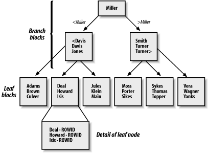
The B*-tree index is composed of one or more levels of branch blocks and a single level of leaf blocks. The branch blocks contain information about the range of values contained in the next level of branch blocks. The number of branch levels between the root and leaf blocks is called the depth of the index. The leaf blocks contain the actual index values and the ROWID for the associated row.
The B*-tree index structure doesn’t contain many blocks at the higher levels of branch blocks, so it takes relatively few I/O operations to read quite far down the B*-tree index structure. All leaf blocks are at the same depth in the index, so all retrievals require essentially the same amount of I/O to get to the index entry, which evens out the performance of the index.
Oracle allows you to create index organized tables (IOTs), in which the leaf blocks store the entire row of data rather than only the ROWID that points to the associated row. Index organized tables reduce the amount of space needed to store an index and a table by eliminating the need to store the ROWID in the leaf page. But index organized tables cannot use a UNIQUE constraint or be stored in a cluster. In addition, index organized tables don’t support distribution, replication, and partitioning (covered in greater detail in other chapters), although IOTs can be used with Oracle Streams for capturing and applying changes with Oracle Database 10g.
There have been a number of enhancements to index organized tables as of Oracle9i, including a lifting of the restriction against the use of bitmap indexes as secondary indexes for an IOT and the ability to create, rebuild, or coalesce secondary indexes on an IOT. Oracle Database 10g continues this trend by allowing list partitioning for index organized tables, as well as providing other enhancements.
Reverse key indexes
Reverse key indexes, as their name implies, automatically reverse the order of the bytes in the key value stored in the index. If the value in a row is “ABCD”, the value for the reverse key index for that row is “DCBA”.
To understand the need for a reverse key index, you have to review some basic facts about the standard B*-tree index. First and foremost, the depth of the B*-tree is determined by the number of entries in the leaf nodes. The greater the depth of the B*-tree, the more levels of branch nodes there are and the more I/O is required to locate and access the appropriate leaf node.
The index illustrated in Figure 4-1 is a nice, well-behaved, alphabetic-based index. It’s balanced, with an even distribution of entries across the width of the leaf pages. But some values commonly used for an index are not so well behaved. Incremental values, such as ascending sequence numbers or increasingly later date values, are always added to the right side of the index, which is the home of higher and higher values. In addition, any deletions from the index have a tendency to be skewed toward the left side as older rows are deleted. The net effect of these practices is that over time the index turns into an unbalanced B*-tree, where the left side of the index is more sparsely populated than the leaf nodes on the right side. This unbalanced growth has the overall effect of increasing the depth of the B*-tree structure due to the number of entries on the right side of the index. The effects described here also apply to the values that are automatically decremented, except that the left side of the B*-tree will end up holding more entries.
You can solve this problem by periodically dropping and recreating the index. However, you can also solve it by using the reverse value index, which reverses the order of the value of the index. This reversal causes the index entries to be more evenly distributed over the width of the leaf nodes. For example, rather than having the values 234, 235, and 236 be added to the maximum side of the index, they are translated to the values 432, 532, and 632 for storage and then translated back when the values are retrieved. These values are more evenly spread throughout the leaf nodes.
The overall result of the reverse index is to correct the imbalance caused by continually adding increasing values to a standard B*-tree index. For more information about reverse key indexes and where to use them, refer to your Oracle documentation.
Bitmap indexes
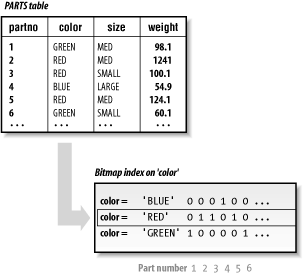
In a standard B*-tree index, the ROWIDs are stored in the leaf blocks of the index. In a bitmap index, each bit in the index represents a ROWID. If a particular row contains a particular value, the bit for that row is “turned on” in the bitmap for that value. A mapping function converts the bit into its corresponding ROWID. Unlike other index types, bitmap indexes include entries for NULL values.
You can store a bitmap index in much less space than a standard B*-tree index if there aren’t many values in the index. Figure 4-2 shows an illustration of how a bitmap index is stored. Figure 9-3 in Chapter 9 shows how a bitmap index is used in a selection condition.
The functionality provided by bitmap indexes is especially important in data warehousing applications in which each dimension of the warehouse contains many repeating values and queries typically require the interaction of several different dimensions. For more about data warehousing, see Chapter 9.
Function-based indexes
Function-based indexes were new in Oracle8i. A function-based index is just like a standard B*-tree or bitmap index, except that you can base the index on the result of a SQL function, rather than just on the value of a column or columns.
Prior to Oracle8i, if you wanted to select on the result of a function, Oracle retrieved every row in the database, executed the function, and then accepted or rejected each row. With function-based indexes you can simply use the index for selection, without having to execute the function on every row, every time.
For example, without a function-based index, if you wanted to perform a case-insensitive selection of data you would have to use the UPPER function in the WHERE clause, which would retrieve every candidate row and execute the function. With a function-based index based on the UPPER function, you can select directly from the index.
Tip
With Oracle Database 10g, you can perform case- or accent-insensitive queries; such queries provide another way to solve this problem.
This capability becomes even more valuable when you consider that you can create your own functions in an Oracle database. You can create a very sophisticated function and then create an index based on the function, which can dramatically affect the performance of queries that require the function.
Additional Data Structures
There are several other data structures available in your Oracle database that can be useful in some circumstances.
Sequences
One of the big problems that occurs in a multiuser database is the difficulty of supplying unique numbers for use as keys or identifiers. For this situation, Oracle allows you to create an object called a sequence. The sequence object is fairly simple. Whenever anyone requests a value from it, it returns a value and increments its internal value, avoiding contention and time-consuming interaction with the requesting application. Oracle can cache a range of numbers for the sequence so that access to the next number doesn’t have to involve disk I/O; rather, it can be satisfied from the range in the SGA.
Sequence numbers are defined with a name, an incremental value, and some additional information about the sequence. Sequences exist independently of any particular table, so more than one table can use the same sequence number.
Consider what might happen if you didn’t use Oracle sequences. You might store the last sequence number used in a column in a table. A user who wanted to get the next sequence number would read the last number, increment it by a fixed value, and write the new value back to the column. But if many users tried to get a sequence number at the same time, they might all read the “last” sequence number before the new “last” sequence number had been written back. You could lock the row in the table with the column containing the sequence number, but this would cause delays as other users waited on locks. What’s the solution? Create a sequence.
Synonyms
All data structures within an Oracle database are stored within a specific schema. A schema is associated with a particular username, and all objects are referenced with the name of the schema followed by the name of the object.
For instance, if there is a table named EMP in a schema named DEMO, the table would be referenced with the complete name of DEMO.EMP. If you don’t supply a specific schema name, Oracle assumes that the structure is in the schema for your current username.
Schemas are a nice feature because object names have to be unique only within their own schemas, but the qualified names for objects can get confusing, especially for end users. To make names simpler and more readable, you can create a synonym for any table, view, snapshot, or sequence, or for any PL/SQL procedure, function, or package.
Synonyms can be either public, which means that all users of a database can use them, or private, which means that only the user whose schema contains the synonym can use it. For example, if the user DEMO creates a public synonym called EMP for the table EMP in his schema, all other users can simply use EMP to refer to the EMP table in DEMO’s schema. Suppose that DEMO didn’t create a public synonym and a user called SCOTT wanted to use the name EMP to refer to the EMP table in DEMO’s schema. The user SCOTT would create a private synonym in his schema. Of course, SCOTT must have access to DEMO’s EMP table for this to work.
Synonyms simplify user access to a data structure. You can also use synonyms to hide the location of a particular data structure, making the data more transportable and increasing the security of the associated table by hiding the name of the schema owner.
Prior to Oracle Database 10g, if you changed the location referenced by a synonym, you would have to recompile any PL/SQL procedures that accessed the synonym.
Clusters
A cluster is a data structure that improves retrieval performance. A cluster, like an index, doesn’t affect the logical view of the table.
A cluster is a way of storing related data values together on disk. Oracle reads data a block at a time, so storing related values together reduces the number of I/O operations needed to retrieve related values, because a single data block will contain only related rows.
A cluster is comprised of one or more tables. The cluster includes a cluster index, which stores all the values for the corresponding cluster key. Each value in the cluster index points to a data block that contains only rows with the same value for the cluster key.
If a cluster contains multiple tables, the tables should be joined together and the cluster index should contain the values that form the basis of the join.
Because the value of the cluster key controls the placement of the rows that relate to the key, changing a value in that key can cause Oracle to change the location of rows associated with that key value.
Clusters may not be appropriate for tables that regularly require full table scans, in which a query requires the Oracle database to iterate through all the rows of the table. Because you access a cluster table through the cluster index, which then points to a data block, full table scans can actually require more I/O operations, lowering overall performance.
Hash Clusters
A hash cluster is like a cluster with one significant difference that can make it even faster: the values for the cluster key are stored in the cluster index. Each request for data in a clustered table involves at least two I/O operations, one for the cluster index and one for the data. A hash cluster stores related data rows together, but groups the rows according to a hash value for the cluster key. The hash value is calculated with a hash function, which means that each retrieval operation starts with a calculation of the hash value and then goes directly to the data block that contains the relevant rows. By eliminating the need to go to a cluster index, a hash clustered table can be even faster for retrieving data than a clustered table. You can control the number of possible hash values for a hash cluster with the HASHKEYS parameter when you create the cluster.
Because the hash cluster directly points to the location of a row in the table, you must allocate all the space required for all the possible values in a hash cluster when you create the cluster.
Hash clusters work best when there is an even distribution of rows among the various values for the hash key. You may have a situation in which there is already a unique value for the hash key column, such as a unique ID. In such situations, you can assign the value for the hash key as the value for the hash function on the unique value, which eliminates the need to execute the hash function as part of the retrieval process. In addition, you can specify your own hash function as part of the definition of a hash cluster.
Oracle Database 10g introduces sorted hash clusters, where data is not only stored in a cluster based on a hash value, but is also stored in the order in which it was inserted. This data structure improves performance for applications that access data in the order in which it was added to the database.
Data Design
Tables and columns present a logical view of the data in a relational database. The flexibility of a relational database gives you many options for grouping the individual pieces of data, represented by the columns, into a set of tables. To use Oracle effectively, you must understand and follow some firmly established principles of database design.
The topic of database design is vast and deep: we won’t even pretend to offer more than a cursory overview. For more information, we recommend the book Oracle Design by Dave Ensor and Ian Stevenson (see Appendix B for details).
When E. F. Codd created the concept of a relational database in the 1960s, he also began work on the concept of normalized data design. The theory behind normalized data design is pretty straightforward: a table should contain only the information that is directly related to the key value of the table. The process of assembling these logical units of information is called normalization of the database design.
The concept of normalized table design was tailored to the capabilities of the relational database. Because you could join data from different tables together in a query, there was no need to keep all the information associated with a particular object together in a single record. You could decompose the information into associated units and simply join the appropriate units together when you needed information that crossed table boundaries.
There are many different methodologies for normalizing data. The following is one example. You start by defining all the data required by your application:
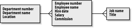
Identify the objects your application needs to know (the entities). Examples of entities, as shown in Figure 4-3, include employees, locations, and jobs.
Identify the individual pieces of data, referred to by data modelers as attributes, for these entities. In Figure 4-3, employee name and salary are attributes. Typically, entities correspond to tables and attributes correspond to columns.
As a potential last step in the process, identify relationships between the entities based on your business. These relationships are implemented in the database schema through the use of structures such as foreign keys. For example, the primary key of the DEPARTMENT NUMBER table would be a foreign key column in the EMPLOYEE NAME table used to identify the DEPARTMENT NUMBER in which an employee works. A foreign key is a type of constraint; constraints are discussed later in this chapter.
Normalization provides benefits by avoiding storage of redundant data. Storing the department in every employee record not only would waste space but would also lead to a data maintenance issue. If the department name changed, you would have to update every employee record, even though no employees had actually changed departments. By normalizing the department data into a table and simply pointing to the appropriate row from the employee rows, you avoid both duplication of data and this type of problem.
However, there is an even more important reason to go through the process of designing a normalized database. You can benefit from normalization because of the planning process that normalizing a data design entails. By really thinking about the way the intended applications use data, you get a much clearer picture of the needs the system is designed to serve. This understanding leads to a much more focused database and application.
Normalization also reduces the amount of data that any one row in a table contains. The less data in a row, the less I/O is needed to retrieve it, which helps to avoid this performance bottleneck. In addition, the smaller the data in a row, the more rows are retrieved per data block, which increases the likelihood that more than one desired row will be retrieved in a single I/O operation. And the smaller the row, the more rows will be kept in Oracle’s system buffers, which also increases the likelihood that a row will be available in memory when it’s needed, thereby avoiding the need for any disk I/O at all.
Finally, the process of normalization includes the creation of foreign key relationships and other data constraints. These relationships build a level of data integrity directly into your database design.
Figure 4-3 shows a simple list of attributes grouped into entities and linked by a foreign key relationship.
Creating a normalized data design isn’t the only data design work you will have to do. Once you’ve completed an optimal logical database design, you must go back and consider what indexes you should add to improve the anticipated performance of the database and whether you should designate any tables as part of a cluster or hash cluster.
Because adding these types of performance-enhancing data structures doesn’t affect the logical representation of the database, you can always make these types of modifications later when you see the way an application uses the database in test mode or in production.
Constraints
A constraint enforces certain aspects of data integrity within a database. When you add a constraint to a particular column, Oracle automatically ensures that data violating that constraint is never accepted. If a user attempts to write data that violates a constraint, Oracle returns an error for the offending SQL statement.
Constraints may be associated with columns when you create or add the table containing the column (via a number of keywords) or after the table has been created with the SQL statement ALTER TABLE. Five constraint types are supported by Oracle8 and later versions:
- NOT NULL
You can designate any column as NOT NULL. If any SQL operation leaves a NULL value in a column with a NOT NULL constraint, Oracle returns an error for the statement.
- Unique
When you designate a column or set of columns as unique, users cannot enter values that already exist in another row in the table for those columns.
The unique constraint is implemented by the creation of an index, which requires a unique value. If you include more than one column as part of a unique key, you will create a single index that will include all the columns in the unique key. If an index already exists for this purpose, Oracle will automatically use that index.
If a column is unique but allows NULL values, any number of rows can have a NULL value, because the NULL indicates the absence of a value. To require a unique value for a column in every row, the column should be both unique and NOT NULL.
- Primary key
Each table can have, at most, a single primary key constraint. The primary key may consist of more than one column in a table.
The primary key constraint forces each primary key to have a unique value. It enforces both the unique constraint and the NOT NULL constraint. A primary key constraint will create a unique index, if one doesn’t already exist for the specified column(s).
- Foreign key
The foreign key constraint is defined for a table (known as the child) that has a relationship with another table in the database (known as the parent). The value entered in a foreign key must be present in a unique or primary key of another specific table. For example, the column for a department ID in an employee table might be a foreign key for the department ID primary key in the department table.
A foreign key can have one or more columns, but the referenced key must have an equal number of columns. You can have a foreign key relate to the primary key of its own table, such as when the employee ID of a manager is a foreign key referencing the ID column in the same table.
A foreign key can contain a NULL value if it’s not forbidden through another constraint.
By requiring that the value for a foreign key exist in another table, the foreign key constraint enforces referential integrity in the database. Foreign keys not only provide a way to join related tables but also ensure that the relationship between the two tables will have the required data integrity.
Normally, you cannot delete a row in a parent table if it causes a row in the child table to violate a foreign key constraint. However, you can specify that a foreign key constraint causes a cascade delete, which means that deleting a referenced row in the parent table automatically deletes all rows in the child table that reference the primary key value in the deleted row in the parent table.
- Check
A check constraint is a more general-purpose constraint. A check constraint is a Boolean expression that evaluates to either TRUE or FALSE. If the check constraint evaluates to FALSE, the SQL statement that caused the result returns an error. For example, a check constraint might require the minimum balance in a bank account to be over $100. If a user tries to update data for that account in a way that causes the balance to drop below this required amount, the constraint will return an error.
Some constraints require the creation of indexes to support them. For instance, the unique constraint creates an implicit index used to guarantee uniqueness. You can also specify a particular index that will enforce a constraint when you define that constraint.
All constraints can be either immediate or deferred. An immediate constraint is enforced as soon as a write operation affects a constrained column in the table. A deferred constraint is enforced when the SQL statement that caused the change in the constrained column completes. Because a single SQL statement can affect several rows, the choice between using a deferred constraint or an immediate constraint can significantly affect how the integrity dictated by the constraint operates. You can specify that an individual constraint is immediate or deferred, or you can set the timing for all constraints in a single transaction.
Finally, you can temporarily suspend the enforcement of constraints for a particular table. When you reenable the operation of the constraint, you can instruct Oracle to validate all the data for the constraint or simply start applying the constraint to the new data. When you add a constraint to an existing table, you can also specify whether you want to check all the existing rows in the table.
Triggers
You use constraints to automatically enforce data integrity rules whenever a user tries to write or modify a row in a table. There are times when you want the same kind of enforcement of your own database or application-specific logic. Oracle includes triggers to give you this capability.
Tip
Although you can write triggers to perform the work of a constraint, Oracle has optimized the operation of constraints, so it’s best to always use a constraint instead of a trigger if possible.
A trigger is a block of code that is fired whenever a particular type of database event occurs to a table. There are three types of events that can cause a trigger to fire:
A database UPDATE
A database INSERT
A database DELETE
You can, for instance, define a trigger to write a customized audit record whenever a user changes a row.
Triggers are defined at the row level. You can specify that a trigger is to be fired either for each row or for the SQL statement that fires the trigger event. As with the previous discussion of constraints, a single SQL statement can affect many rows, so the specification of the trigger can have a significant effect on the operation of the trigger and the performance of the database.
There are three times when a trigger can fire:
Before the execution of the triggering event
After the execution of the triggering event
Instead of the triggering event
Combining the first two timing options with the row and statement versions of a trigger gives you four possible trigger implementations: before a statement, before a row, after a statement, and after a row.
INSTEAD OF triggers were introduced with Oracle8. The INSTEAD OF trigger has a specific purpose: to implement data-manipulation operations on views that don’t normally permit them, such as a view that references columns in more than one base table for updates. You should be careful when using INSTEAD OF triggers because of the many potential problems associated with modifying the data in the underlying base tables of a view. There are many restrictions on when you can use INSTEAD OF triggers. Refer to your Oracle documentation for a detailed description of the forbidden scenarios.
You can specify a trigger restriction for any trigger. A trigger restriction is a Boolean expression that circumvents the execution of the trigger if it evaluates to FALSE.
Triggers are defined and stored separately from the tables that use them. Because they contain logic, they must be written in a language with capabilities beyond those of SQL, which is designed to access data. Oracle8 and later versions allow you to write triggers in PL/SQL, the procedural language that has been a part of Oracle since Version 6. Oracle8i and beyond also support Java as a procedural language, so you can create Java triggers with those versions.
You can write a trigger directly in PL/SQL or Java, or a trigger can call an existing stored procedure written in either language.
Triggers are fired as a result of a SQL statement that modifies a row in a particular table. It’s possible for the actions of the trigger to modify the data in the table or to cause changes in other tables that fire their own triggers. The end result of this may be data that ends up being changed in a way that Oracle thinks is logically illegal. These situations can cause Oracle to return runtime errors referring to mutating tables, which are tables modified by other triggers, or constraining tables, which are tables modified by other constraints. Oracle8i eliminated some of the errors caused by activating constraints with triggers.
Oracle8i also introduced a very useful set of system event triggers (sometimes called database-level event triggers), and user event triggers (sometimes called schema-level event triggers). You can now place a trigger on system events such as database startup and shutdown and on user events such as logging on and logging off.
Query Optimization
All of the data structures discussed so far in this chapter are server entities. Users request data from an Oracle server through database queries. Oracle’s query optimizer must then determine the best way to access the data requested by each query.
One of the great virtues of a relational database is its ability to access data without predefining the access paths to the data. When a SQL query is submitted to an Oracle database, Oracle must decide how to access the data. The process of making this decision is called query optimization, because Oracle looks for the optimal way to retrieve the data. This retrieval is known as the execution path. The trick behind query optimization is to choose the most efficient way to get the data, because there may be many different options available.
For instance, even with a query that involves only a single table, Oracle can take either of these approaches:
Although it’s usually much faster to retrieve data using an index, the process of getting the values from the index involves an additional I/O step in processing the query. Query optimization may be as simple as determining whether the query involves selection conditions that can be imposed on values in the index. Using the index values to select the desired rows involves less I/O and is therefore more efficient than retrieving all the data from the table and then imposing the selection conditions.
Another factor in determining the optimal query execution plan is whether there is an ORDER BY condition in the query that can be automatically implemented by the presorted index. Alternatively, if the table is small enough, the optimizer may decide to simply read all the blocks of the table and bypass the index because it estimates the cost of the index I/O plus the table I/O to be higher than just the table I/O.
The query optimizer has to make some key decisions even with a query on a single table. When a more involved query is submitted, such as one involving many tables that must be joined together efficiently or one that has a complex selection criteria and multiple levels of sorting, the query optimizer has a much more complex task.
Prior to Oracle Database 10g, you could choose between two different Oracle query optimizers, a rule-based optimizer and a cost-based optimizer, which are described in the following sections. With Oracle Database 10g, the rule-based optimizer is desupported. The references to syntax and operations for the rule-based optimizer in the following sections are provided as a convenience and are applicable only if you are running an older release of Oracle.
Rule-Based Optimization
Oracle has always had a query optimizer, but until Oracle7 the optimizer was only rule-based. The rule-based optimizer, as the name implies, uses a set of predefined rules as the main determinant of query optimization decisions. As noted earlier, the rule-based optimizer is desupported in Oracle Database 10g.
Rule-based optimization was sometimes a better choice than other random methods of optimization or the Oracle cost-based optimizer in early Oracle releases, despite some significant weaknesses. One weakness is the simplistic set of rules. The Oracle rule-based optimizer has about twenty rules and assigns a weight to each one of them. In a complex database, a query can easily involve several tables, each with several indexes and complex selection conditions and ordering. This complexity means that there will be a lot of options, and the simple set of rules used by the rule-based optimizer might not differentiate the choices well enough to make the best choice.
The rule-based optimizer assigns an optimization score to each potential execution path and then takes the path with the best optimization score. Another main weakness of the rule-based optimizer stems from the way it resolved optimization choices made in the event of a “tie” score. When two paths present the same optimization score, the rule-based optimizer looks to the syntax of the SQL statement to resolve the tie. The winning execution path is based on the order in which the tables occur in the SQL statement.
You can understand the potential impact of this type of tie-breaker by looking at a simple situation in which a small table with 10 rows, SMALLTAB, is joined to a large table with 10,000 rows, LARGETAB, as shown in Figure 4-4. If the optimizer chooses to read SMALLTAB first, the Oracle database will read the 10 rows and then read LARGETAB to find the matching rows for all 10 of these rows. If the optimizer chooses to read LARGETAB first, the database will read 10,000 rows from LARGETAB and then read SMALLTAB 10,000 times to find the matching rows. Of course, the rows in SMALLTAB will probably be cached, thus reducing the impact of each probe, but the two optimizer choices still offer a dramatic difference in potential performance.
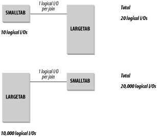
Differences like this occur as a result of the ordering of the table names in the query. In the previous situation the rule-based optimizer returns the same results for the query, but it uses widely varying amounts of resources to retrieve those results.
Cost-Based Optimization
To improve the optimization of SQL statements, Oracle introduced the cost-based optimizer in Oracle7. As the name implies, the cost-based optimizer does more than simply look at a set of optimization rules; instead, it selects the execution path that requires the least number of logical I/O operations. This approach avoids the error discussed in the previous section. After all, the cost-based optimizer would know which table was bigger and would select the right table to begin the query, regardless of the syntax of the SQL statement.
Oracle8 and later versions, by default, attempt to use the cost-based optimizer to identify the optimal execution plan. As we’ve mentioned, in Oracle Database 10g, the cost-based optimizer is the only supported choice. To properly evaluate the cost of any particular execution plan, the cost-based optimizer uses statistics about the composition of the relevant data structures. These statistics are automatically gathered in Oracle Database 10g.
Statistics
Like the rule-based optimizer, the cost-based optimizer finds the optimal execution plan by assigning an optimization score for each of the potential execution plans. However, the cost-based optimizer uses its own internal rules and logic along with statistics that reflect the state of the data structures in the database. These statistics relate to the tables, columns, and indexes involved in the execution plan. The statistics for each type of data structure are listed in Table 4-1.
Oracle Database 10g also collects overall system statistics, including I/O and CPU performance and utilization.
These statistics are stored in three tables in the data dictionary, which are described in the final section of this chapter, Section 4.10.
|
Data structure |
Type of statistics |
|
Table |
Number of rows Number of blocks Number of unused blocks Average available free space per block Number of chained rows Average row length |
|
Column |
Number of distinct values per column Second-lowest column value Second-highest column value Column density factor |
|
Index |
Depth of index B*-tree structure Number of leaf blocks Number of distinct values Average number of leaf blocks per key Average number of data blocks per key Clustering factor |
You can see that these statistics can be used individually and in combination to determine the overall cost of the I/O required by an execution plan. The statistics reflect both the size of a table and the amount of unused space within the blocks; this space can, in turn, affect how many I/O operations are needed to retrieve rows. The index statistics reflect not only the depth and breadth of the index tree, but also the uniqueness of the values in the tree, which can affect the ease with which values can be selected using the index.
Oracle8 and later versions use the SQL statement ANALYZE to collect these statistics. (This is no longer needed in Oracle Database 10g because statistics can be gathered automatically.) You can analyze a table, an index, or a cluster in a single SQL statement. Collecting statistics can be a resource-intensive job; in some ways, it’s like building an index. Because of its potential impact, the ANALYZE command has two options:
The latter choice makes gathering the relative statistics for the data structure consume far fewer resources than computing the exact figures for the entire structure. If you have a very large table, for example, analyzing 5% or less of the table will probably produce an accurate estimate of the relative percentages of unused space and other relative data.
Tip
The accuracy of the cost-based optimizer depends on the accuracy of the statistics it uses, so you should make updating statistics a standard part of your maintenance plan. With Oracle Database 10g, you can enable automatic statistics collection for a table, which can be based on whether a table is either stale (which means that more than 10% of the objects in the table have changed) or empty.
The use of statistics makes it possible for the cost-based optimizer to make a much more well-informed choice of the optimal execution plan. For instance, the optimizer could be trying to decide between two indexes to use in an execution plan that involves a selection based on a value in either index. The rule-based optimizer might very well rate both indexes equally and resort to the order in which they appear in the WHERE clause to choose an execution plan. The cost-based optimizer, however, knows that one index contains 1,000 entries while the other contains 10,000 entries. It even knows that the index that contains 1,000 values contains only 20 unique values, while the index that contains 10,000 values has 5,000 unique values. The selectivity offered by the larger index is much greater, so that index will be assigned a better optimization score and used for the query.
In Oracle9i, you have the option of allowing the cost-based optimizer to use CPU speed as one of the factors in determining the optimal execution plan. An initialization parameter turns this feature on and off. In Oracle Database 10g, the default cost basis is calculated on the CPU cost plus the I/O cost for a plan.
Even with all the information available to it, the cost-based optimizer did have some noticeable initial flaws. Aside from the fact that it (like all software) occasionally has bugs, the cost-based optimizer used statistics that didn’t provide a complete picture of the data structures. In the previous example, the only thing the statistics tell the optimizer about the indexes is the number of distinct values in each index. They don’t reveal anything about the distribution of those values. For instance, the larger index can contain 5,000 unique values, but these values can each represent two rows in the associated table, or one index value can represent 5,001 rows while the rest of the index values represent a single row. The selectivity of the index can vary wildly, depending on the value used in the selection criteria of the SQL statement. Fortunately, Oracle 7.3 introduced support for collecting histogram statistics for indexes to address this exact problem. You create histograms using syntax within the ANALYZE INDEX statement when you gather statistics yourself in Oracle versions prior to Oracle Database 10g. This syntax is described in your Oracle SQL reference documentation.
Oracle8 and more recent releases come with a built-in PL/SQL package, DBMS_STATS, which contains a number of procedures that can help you to automate the process of collecting statistics. Many of the procedures in this package also collect statistics with parallel operations, which can speed up the collection process.
Influencing the cost-based optimizer
There are two ways you can influence the way the cost-based optimizer selects an execution plan. The first way is by setting the optimizer mode to favor either batch- type requests or interactive requests with the ALL_ROWS or FIRST_ROWS choice.
You can set the optimizer mode to weigh the options for the execution plan to either favor ALL_ROWS, meaning the overall time that it takes to complete the execution of the SQL statement, or FIRST_ROWS, meaning the response time for returning the first set of rows from a SQL statement. The optimizer mode tilts the evaluation of optimization scores slightly and, in some cases, may result in a different execution plan. ALL_ROWS and FIRST_ROWS are two of four choices for the optimizer mode, which is described in more detail in the next section.
Oracle also gives you a way to completely override the decisions of the optimizer with a technique called hints. A hint is nothing more than a comment with a specific format inside a SQL statement. You can use hints to force a variety of decisions onto the optimizer, such as:
Use of the rule-based optimizer prior to Oracle Database 10g
Use of a full table scan
Use of a particular index
Use of a specific number of parallel processes for the statement
Hints come with their own set of problems. A hint looks just like a comment, as shown in this extremely simple SQL statement. Here, the hint forces the optimizer to use the EMP_IDX index for the EMP table:
SELECT /*+ INDEX(EMP_IDX) */ LASTNAME, FIRSTNAME, PHONE FROM EMP
If a hint isn’t in the right place in the SQL statement, if the hint keyword is misspelled, or if you change the name of a data structure so that the hint no longer refers to an existing structure, the hint will simply be ignored, just as a comment would be. Because hints are embedded into SQL statements, repairing them can be quite frustrating and time-consuming if they aren’t working properly. In addition, if you add a hint to a SQL statement to address a problem caused by a bug in the cost-based optimizer and the cost-based optimizer is subsequently fixed, the SQL statement is still outside the scope of the optimization calculated by the optimizer.
However, hints do have a place—for example, when a developer has a user-defined datatype that suggests a particular type of access. The optimizer cannot anticipate the effect of user-defined datatypes, but a hint can properly enable the appropriate retrieval path.
Tip
Since Oracle9i, you can extend the optimizer to include user-defined function and domain-based indexes as part of the optimization process.
For more details about when hints might be considered, see the sidebar “Accepting the Verdict of the Optimizer” later in this chapter.
Choosing a Mode
In the previous section we mentioned two optimizer modes: ALL_ROWS and FIRST_ROWS. The two other valid optimizer modes for all Oracle versions prior to Oracle Database 10g are:
- RULE
Forces the use of the rule-based optimizer
- CHOOSE
Allows Oracle to choose whether to use the cost-based optimizer or the rule-based optimizer
With an optimizer mode of CHOOSE, which is the default setting, Oracle will use the cost-based optimizer if any of the tables in the SQL statement have statistics associated with them. The cost-based optimizer will make a statistical estimate for the tables that lack statistics. It’s important to understand that partially collected statistics can cause tremendous problems. If one of the tables in a SQL statement has statistics, Oracle will use the cost-based optimizer. If the optimizer is acting on incomplete information, the quality of optimization will suffer accordingly. If you’re going to use the cost-based optimizer, make sure you gather complete statistics for your databases.
You can set the optimizer level at the instance level, at the session level, or within an individual SQL statement. But the big question remains, especially for those of you who have been using Oracle since before the introduction of the cost-based optimizer: which optimizer should I choose?
Why choose the cost-based optimizer?
We favor using the cost-based optimizer, even prior to Oracle Database 10g, for several reasons.
First, the cost-based optimizer makes decisions with a wider range of knowledge about the data structures in the database. Although the cost-based optimizer isn’t flawless in its decision-making process, it does tend to make more accurate decisions based on its wider base of information, especially because it has been around since Oracle7 and has been improved with each new release.
Second, the cost-based optimizer has been enhanced to take into account improvements in the Oracle database itself, while the rule-based optimizer has not. For instance, the cost-based optimizer understands the impact that partitioned tables have on the selection of an execution plan, while the rule-based optimizer does not. As another example, the cost-based optimizer can optimize execution plans for star schema queries, which are heavily used in data warehousing, while the rule-based optimizer has not been enhanced to deal effectively with these types of queries.
The reason for this bias is simple: Oracle Corporation has been quite frank about their intention to make the cost-based optimizer the optimizer for the Oracle database. Oracle hasn’t been adding new features to the rule-based optimizer and hasn’t guaranteed support for it in future releases. As we have mentioned, with Oracle Database 10g, the rule-based optimizer is no longer supported
So your future (or your present, with Oracle Database 10g) lies in the cost-based optimizer. But there are still situations in which you might want to use the rule-based optimizer if you are running a release of Oracle prior to Oracle Database 10g.
Why choose the rule-based optimizer?
As the old saying goes, if it ain’t broke, don’t fix it. And you may be in an environment in which you’ve designed and tuned your SQL to operate optimally with the rule-based optimizer. Although you should still look ahead to a future in which only the cost-based optimizer is supported, there may be no reason to switch over to the cost-based optimizer now if you have an application that is already performing at its best and you are not planning to move to Oracle Database 10g in the near term.
The chances are pretty good that the cost-based optimizer will choose the same execution plan as a properly tuned application using the rule-based optimizer. But there is always a chance that the cost-based optimizer will make a different choice, which can create more work for you, because you might have to spend time tracking down the different optimizations.
Remember the bottom line for all optimizers: no optimizer can provide a performance increase for a SQL statement that’s already running optimally. The cost-based optimizer is not a magic potion that remedies the problems brought on by a poor database and application design or an inefficient implementation platform.
The good news is that Oracle gives you a lot of flexibility in accepting, storing, or overriding the verdict of the optimizer.
Saving the Optimization
There may be times when you want to prevent the optimizer from calculating a new plan whenever a SQL statement is submitted. For example, you might do this if you’ve finally reached a point at which you feel the SQL is running optimally, and you don’t want the plan to change regardless of future changes to the optimizer or the database.
Starting with Oracle8i, you can create a stored outline that will store the attributes used by the optimizer to create an execution plan. Once you have a stored outline, the optimizer simply uses the stored attributes to create an execution plan. With Oracle9i, you can also edit the hints that make up a stored outline.
Remember that storing an outline fixes the optimization of the outline at the time the outline was stored. Any subsequent improvements to the optimizer will not affect the stored outlines, so you should document your use of stored outlines and consider restoring them with new releases.
Understanding the Execution Plan
Oracle’s query optimizer automatically selects an execution plan for each query submitted. By and large, although the optimizer does a good job of selecting the execution plan, there may be times when the performance of the database suggests that it’s using a less-than-optimal execution plan.
The only way you can really tell what path is being selected by the optimizer is to see the layout of the execution plan. You can use two Oracle character-mode utilities to examine the execution plan chosen by the Oracle optimizer, or you can look at the execution plan in Enterprise Manager, as of Oracle Database 10g. These tools allow you to see the successive steps used by Oracle to collect, select, and return the data to the user.
The first utility is the SQL EXPLAIN PLAN statement. When you use EXPLAIN PLAN, followed by the keyword FOR and the SQL statement whose execution plan you want to view, the Oracle cost-based optimizer returns a description of the execution plan it will use for the SQL statement and inserts this description into a database table. You can subsequently run a query on that table to get the execution plan, as shown in SQL*Plus in Figure 4-5.
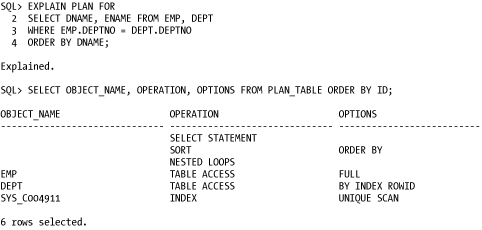
The execution plan is presented as a series of rows in the table, one for each step taken by Oracle in the process of executing the SQL statement. The optimizer also includes some of the information related to its decisions, such as the overall cost of each step and some of the statistics that it used to make its decisions.
The optimizer writes all of this information to a table in the database. By default, the optimizer uses a table called PLAN_TABLE; make sure the table exists before you use EXPLAIN PLAN. (The utlxplan.sql script included with your Oracle database creates the default PLAN_TABLE table.) You can specify that EXPLAIN PLAN uses a table other than PLAN_TABLE in the syntax of the statement. For more information about the use of EXPLAIN PLAN, please refer to your Oracle documentation.
There are times when you want to examine the execution plan for a single statement. In such cases, the EXPLAIN PLAN syntax is appropriate. There are other times when you want to look at the plans for a group of SQL statements. For these situations, you can set up a trace for the statements you want to examine and then use the second utility, TKPROF, to give you the results of the trace in a more readable format in a separate file.
You must use the EXPLAIN keyword when you start TKPROF, as this will instruct the utility to execute an EXPLAIN PLAN statement for each SQL statement in the trace file. You can also specify how the results delivered by TKPROF are sorted. For instance, you can have the SQL statements sorted on the basis of the physical I/Os they used; the elapsed time spent on parsing, executing, or fetching the rows; or the total number of rows affected.
The TKPROF utility uses a trace file as its raw material. Trace files are created for individual sessions. You can start collecting a trace file either by running the target application with a switch (if it’s written with an Oracle product such as Developer) or by explicitly turning it on with an EXEC SQL call or an ALTER SESSION SQL statement in an application written with a 3GL. The trace process, as you can probably guess, can significantly affect the performance of an application, so you should turn it on only when you have some specific diagnostic work to do.
You can also view the execution plan through Enterprise Manager for the SQL statements that use the most resources.
Tuning your SQL statements isn’t a trivial task, but with the EXPLAIN PLAN and TKPROF utilities you can get to the bottom of the decisions made by the cost-based optimizer. It takes a bit of work to understand exactly how to read an execution plan, but it’s better to have access to this type of information than not. In large-scale system-development projects, it’s quite common for developers to submit EXPLAIN PLANs for the SQL they’re writing to a DBA as a formal step toward completing a form or report. While time-consuming, this is the best way to ensure that your SQL is tuned before going into production.
SQL Tuning Advisor
Oracle Database 10g includes a new tool called the SQL Tuning Advisor. This tool performs advanced optimization analysis on selected SQL statements, using workloads that have been automatically collected into the Automatic Workload Repository (AWR) or that you have specified yourself. Once the optimization is done, the SQL Tuning Advisor makes recommendations, which could include updating statistics, adding indexes, or creating an SQL Profile. This Profile is stored in the database and is used as the optimization plan for future executions of the statement, which allows you to “fix” errant SQL plans without having to touch the underlying SQL.
Data Dictionary Tables
The main purpose of the Oracle data dictionary is to store data that describes the structure of the objects in the Oracle database. Because of this purpose, there are many views in the Oracle data dictionary that provide information about the attributes and composition of the data structures within the database.
All of the views listed in this section actually have three varieties, which are identified by their prefixes:
- DBA_
Includes all the objects in the database. A user must have DBA privileges to use this view.
- USER_
Includes only the objects in the user’s own database schema.
- ALL_
Includes all the objects in the database to which a particular user has access. If a user has been granted rights to objects in another user’s schema, these objects will appear in this view.
This means that, for instance, there are three views that relate to tables: DBA_ TABLES, ALL_TABLES, and USER_TABLES.
Some of the more common views that directly relate to the data structures are described in Table 4-2.
|
Data dictionary view |
Type of information |
|
ALL_TABLES |
Information about the object and relational tables |
|
TABLES |
Information about the relational tables |
|
TAB_COMMENTS |
Comments about the table structures |
|
TAB_HISTOGRAMS |
Statistics about the use of tables |
|
TAB_PARTITIONS |
Information about the partitions in a partitioned table |
|
TAB_PRIVS* |
Different views detailing all the privileges on a table, the privileges granted by the user, and the privileges granted to the user |
|
TAB_COLUMNS |
Information about the columns in tables and views |
|
COL_COMMENTS |
Comments about individual columns |
|
COL_PRIVS* |
Different views detailing all the privileges on a column, the privileges granted by the user, and the privileges granted to the user |
|
LOBS |
Information about large object (LOB) datatype columns |
|
VIEWS |
Information about views |
|
INDEXES |
Information about the indexes on tables |
|
IND_COLUMNS |
Information about the columns in each index |
|
IND_PARTITIONS |
Information about each partition in a partitioned index |
|
PART_* |
Different views detailing the composition and usage patterns for partitioned tables and indexes |
|
CONS_COLUMNS |
Information about the columns in each constraint |
|
CONSTRAINTS |
Information about constraints on tables |
|
SEQUENCES |
Information about sequence objects |
|
SYNONYMS |
Information about synonyms |
|
TAB_COL_STATISTICS |
The statistics used by the cost-based optimizer |
|
TRIGGERS |
Information about the triggers on tables |
|
TRIGGER_COLS |
Information about the columns in triggers |
Get Oracle Essentials, 3rd Edition now with the O’Reilly learning platform.
O’Reilly members experience books, live events, courses curated by job role, and more from O’Reilly and nearly 200 top publishers.

