Oracle SQL*Plus: The Definitive Guide, 2nd Edition

Grouping and Summarizing

SQL allows you to divide the rows returned by a query into groups, summarize the data within each group using a special class of functions known as aggregate functions , and return only one row per group. For example, you can count the number of rows in a table using the COUNT function shown in Example 4-28.

Example 4-28. Summarizing data using an aggregate function

               SELECT COUNT(*), COUNT(employee_termination_date)
               FROM employee;

  COUNT(*) COUNT(EMPLOYEE_TERMINATION_DATE)
---------- --------------------------------
        11                                6

There's nothing in Example 4-28 to divide the data being retrieved into groups, so all 11 rows in the employee table are treated as one group. The COUNT function is an aggregate function that can count the number of values or rows in a group. COUNT is special in that you can pass it an asterisk (*) when you wish to count rows. The first use of COUNT in the example shows that the table contains 11 rows. The second use counts the number of values in the employee_termination_date column. Nulls are not counted because nulls represent the absence of value. While there are 11 employees on file, only five are currently employed; the other six have been terminated. This is the kind of business information you can obtain by summarizing your data.

The GROUP BY Clause

You'll rarely want to summarize data across an entire table. More often, you'll find yourself dividing your data into groups. For example, you might wish to group employees by the decade in which they were hired, and then ask the following question: How many employees from each decade are still employed? Example 4-29 shows how to do this.

Example 4-29. Counting the remaining employees from each decade

                  SELECT SUBSTR(TO_CHAR(employee_hire_date,'YYYY'),1,3) || '0' "decade",
                         COUNT(employee_hire_date) "hired",
                         COUNT(employee_hire_date) - COUNT(employee_termination_date) 
                  "remaining",
                         MIN(employee_hire_date) "first hire",
                         MAX(employee_hire_date) "last hire"
                  FROM employee
                  GROUP BY SUBSTR(TO_CHAR(employee_hire_date,'YYYY'),1,3) || '0';

decade             hired  remaining first hire  last hire
------------- ---------- ---------- ----------- -----------
1960                   3          1 15-Nov-1961 16-Sep-1964
1970                   1          1 23-Aug-1976 23-Aug-1976
1980                   1          0 29-Dec-1987 29-Dec-1987
1990                   1          0 01-Mar-1994 01-Mar-1994
2000                   5          3 02-Jan-2004 15-Jun-2004

In addition to COUNT, the example shows the MIN and MAX functions being used to return the earliest and latest hire dates within each group, i.e., within each decade. You can see that five employees were hired in the 2000s, with all five hires occurring between January and June 2004. Two of those new hires have since left the company. By contrast, you have no attrition of people hired during the 1980s and 1990s. Perhaps you should investigate to see whether your Human Resources department is slipping in its hiring practices!

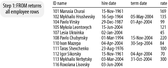
It's worth going into some detail about how GROUP BY queries execute. You should have a correct understanding of these queries. To begin, Figure 4-6 shows all the employee rows as returned by the FROM clause.

Figure 4-6. The FROM operation returns all employee rows

The GROUP BY clause then divides employees into groups by decade, as shown in Figure 4-7. The TO_CHAR function returns the four-digit year of each employee's hire date as a character string. The SUBSTR function extracts the first through third digits from that string, and the || operator is used to replace the fourth digit with a zero. Thus, all years in the range 1960-1969 are transformed into the string "1960." (Appendix B provides more detail about applying TO_CHAR to dates.)

Figure 4-7. The GROUP BY operation divides rows into groups

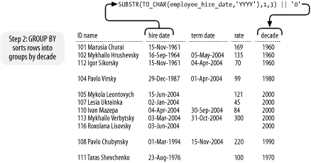
The grouping of rows is often accomplished via a sorting operation. But as Figure 4-7 illustrates, the sort may be incomplete. Don't count on GROUP BY to sort your output. Always use ORDER BY if you want results in a specific order.

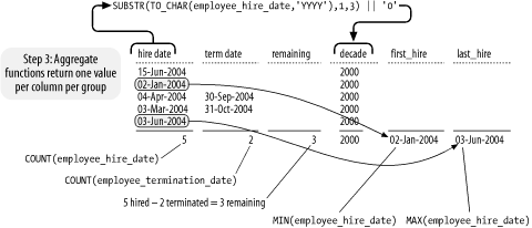
Once the rows are divided into groups, the aggregate functions are applied in order to return just one value per group. Figure 4-8 illustrates this process for just the one group of rows representing the decade 2000.

Figure 4-8. Aggregate functions are applied to return one row per group

There is one column returned by the SELECT statement in Example 4-29 to which an aggregate function has not been applied. That column is the computed column that returns the decade in which an employee was hired. Because that column is the basis by which employees are divided into groups, it makes sense to return it, so you can know to which group each summary row applies. If you omit the decade column, the results in the example will become useless. It's a good idea to identify each summary row by including the GROUP BY columns in the query results.

Warning

All columns other than those listed in the GROUP BY clause must have an aggregate function applied to them. You cannot, for example, return individual employee IDs from the query shown in Example 4-29. You must apply an aggregate function to compute just one value per column, per group.

Example 4-29 uses COUNT(employee_hire_date) as a proxy for the number of employees hired in each decade. This is reasonable because the example database design precludes nulls in the hire date column. Things change, though, if null hire dates are a possibility. If null hire dates were to exist in the data, then those nulls would propagate throughout the decade calculation, and you'd end up with a single group having all the null hire dates. COUNT will not count null values, so the application of COUNT(employee_hire_date) to a group of rows with all null hire dates would result in the value zero. Furthermore, you might have termination dates in that group, so the result of COUNT(employee_termination_date) might be greater than zero. Among all your other output then, you might end up with an oddball result row like the following:

decade             hired  remaining first hir last hire
------------- ---------- ---------- --------- ---------
NULL                   0         -1 NULL      NULL

In this case, you might be better off using COUNT(*) to count rows rather than non-null values. However, that's fixing a symptom. It might make the math look better in the results, but it does nothing to address the underlying problem of bad data. The real fix is to dig into your data and find out why you didn't record hire dates for some of your employees.

The HAVING Clause

You may not want all the summary rows returned by a GROUP BY query. You know that you can use WHERE to eliminate detail rows returned by a regular query. With summary queries, you can use the HAVING clause to eliminate summary rows. Example 4-30 shows a GROUP BY query that uses HAVING to restrict the results to only those employees having logged more than 20 hours toward projects 1001 and 1002.

Example 4-30. HAVING allows you to filter out summary rows that you do not want

                  SELECT employee_id, project_id
                  FROM project_hours
                  GROUP BY employee_id, project_id
                  HAVING (project_id = 1001 OR project_id=1002)
                     AND SUM(hours_logged) > 20;

EMPLOYEE_ID PROJECT_ID
----------- ----------
        101       1002
        107       1002
        108       1002
        111       1002

Notice the use of SUM(hours_logged) to compute the total number of hours each employee has charged to each project. This expression appears only in the HAVING clause, where it is used to restrict output to only those employee/project combinations representing more than 20 hours of work. If you want to see the sum, you can put the expression in the SELECT clause as well, but you're not required to do that.

Example 4-30 is in part a good example of how not to use the HAVING clause. HAVING executes after all the sorting and summarizing of GROUP BY. Any condition you write in the HAVING clause should depend on summarized results. Two conditions in Example 4-30s HAVING clause do not depend on summary calculations. Those conditions should be moved to the WHERE clause, as shown in Example 4-31.

Example 4-31. Put non-summary conditions in the WHERE clause

                  SELECT employee_id, project_id
                  FROM project_hours
                  WHERE project_id = 1001 OR project_id=1002
                  GROUP BY employee_id, project_id
                  HAVING SUM(hours_logged) > 20;

EMPLOYEE_ID PROJECT_ID
----------- ----------
        101       1002
        107       1002
        108       1002
        111       1002

The reason you put all detail-based conditions in the WHERE clause is that the WHERE clause is evaluated prior to the grouping and summarizing operation of GROUP BY. The fewer the rows that have to be sorted, grouped, and summarized, the better your query's performance will be, and the less the load on the database server. Examples Example 4-30 and Example 4-31 produce the same results, but Example 4-31 is more efficient because it eliminates many rows earlier in the query execution process.