Practical Machine Learning for Computer Vision

Chapter 4. Object Detection and Image Segmentation

So far in this book, we have looked at a variety of machine learning architectures but used them to solve only one type of problem—that of classifying (or regressing) an entire image. In this chapter, we discuss three new vision problems: object detection, instance segmentation, and whole-scene semantic segmentation (Figure 4-1). Other more advanced vision problems like image generation, counting, pose estimation, and generative models are covered in Chapters 11 and 12.

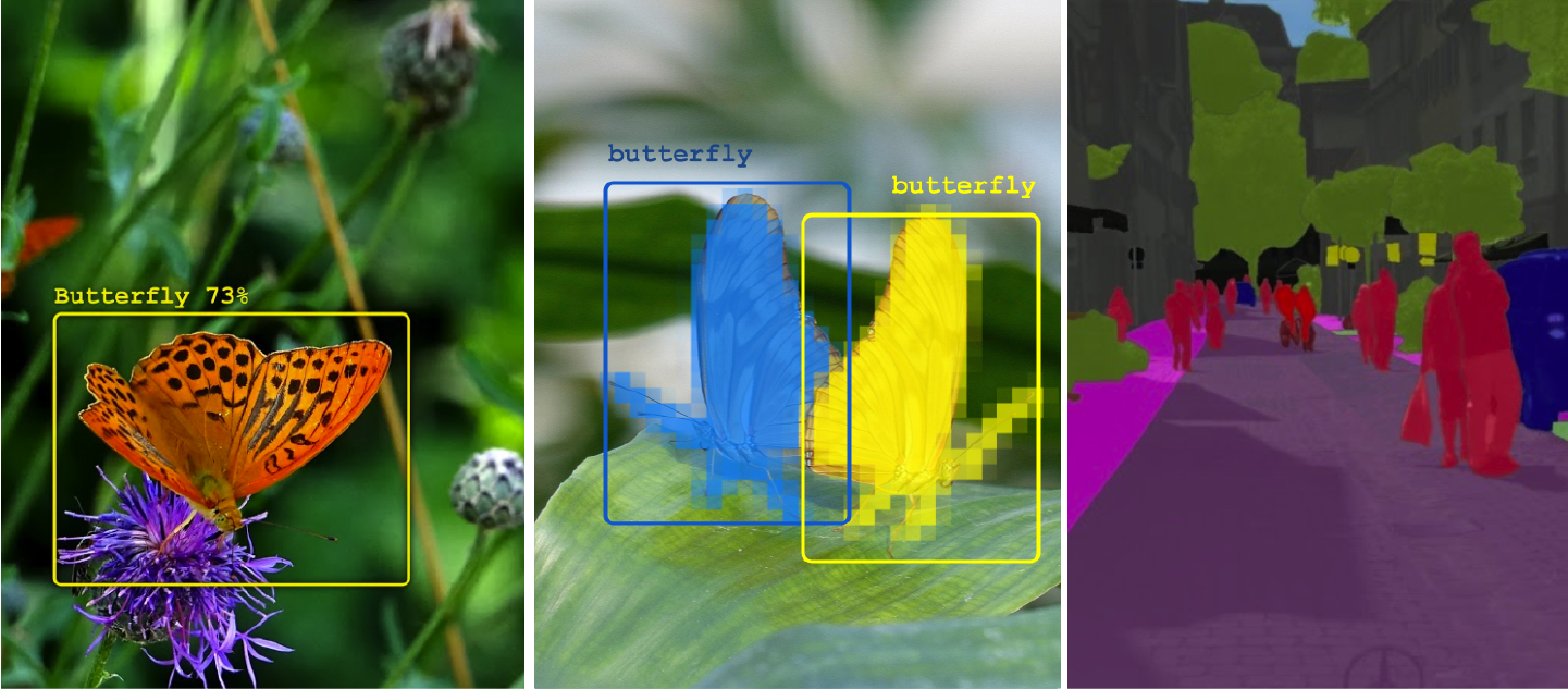
Figure 4-1. From left to right: object detection, instance segmentation, and whole-scene semantic segmentation. Images from Arthropods and Cityscapes datasets.

Tip

The code for this chapter is in the 04_detect_segment folder of the book’s GitHub repository. We will provide file names for code samples and notebooks where applicable.

Object Detection

Seeing is, for most of us, so effortless that, as we glimpse a butterfly from the corner of our eye and turn our head to enjoy its beauty, we don’t even think about the millions of visual cells and neurons at play, capturing light, decoding the signals, and processing them into higher and higher levels of abstraction.

We saw in Chapter 3 how image recognition in ML works. However, the models presented in that chapter were built to classify an image as whole—they could not tell us where in the image a flower was. In this section, we will look at ways to build ML models that can provide this location information. This is a task known as object detection (Figure 4-2).

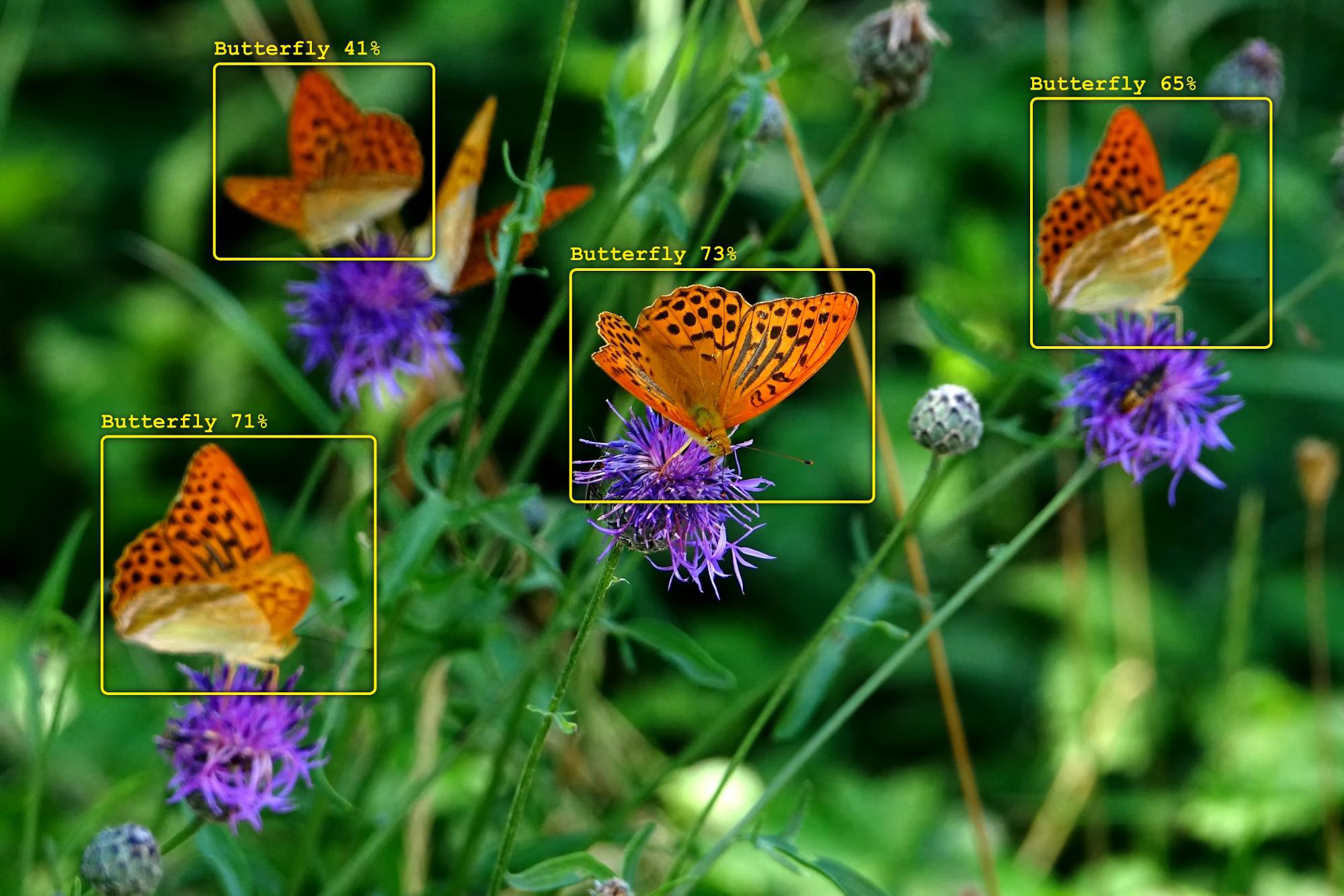
Figure 4-2. An object detection task. Image from Arthropods dataset.

In fact, convolutional layers do identify and locate the things they detect. The convolutional backbones from Chapter 3 already extract some location information. But in classification problems, the networks make no use of this information. They are trained on an objective where location does not matter. A picture of a butterfly is classified as such wherever the butterfly appears in the image. On the contrary, for object detection, we will add elements to the convolutional stack to extract and refine the location information and train the network to do so with maximum accuracy.

The simplest approach is to add something to the end of a convolutional backbone to predict bounding boxes around detected objects. That’s the YOLO (You Only Look Once) approach, and we will start there. However, a lot of important information is also contained at intermediate levels in the convolutional backbone. To extract it, we will build more complex architectures called feature pyramid networks (FPNs) and illustrate their use with RetinaNet.

In this section, we will be using the Arthropod Taxonomy Orders Object Detection dataset (Arthropods for short), which is freely available on Kaggle.com. The dataset contains seven categories—Coleoptera (beetles), Aranea (spiders), Hemiptera (true bugs), Diptera (flies), Lepidoptera (butterflies), Hymenoptera (bees, wasps, and ants), and Odonata (dragonflies)—as well as bounding boxes. Some examples are shown in Figure 4-3.

Figure 4-3. Some examples from the Arthropods dataset for object detection.

Besides YOLO, this chapter will also address the RetinaNet and Mask R-CNN architectures. Their implementations can be found in the TensorFlow Model Garden’s official vision repository. We will be using the new implementations located, at the time of writing, in the “beta” folder of the repository.

Example code showing how to apply these detection models on a custom dataset such as Arthropods can be found in 04_detect_segment on GitHub, in the folder corresponding to Chapter 4.

In addition to the TensorFlow Model Garden, there is also an excellent step-by-step implementation of RetinaNet on the keras.io website.

YOLO

YOLO (you only look once) is the simplest object detection architecture. It is not the most accurate, but it’s one of the fastest when it comes to prediction times. For that reason, it is used in many real-time systems like security cameras. The architecture can be based on any convolutional backbone from Chapter 3. Images are processed through the convolutional stack as in the image classification case, but the classification head is replaced with an object detection and classification head.

More recent variations of the YOLO architecture exist (YOLOv2, YOLOv3, YOLOv4), but we will not be covering them here. We will use YOLOv1 as our first stepping-stone into object detection architectures, because it is the simplest one to understand.

YOLO grid

YOLOv1 (hereafter referred to as “YOLO” for simplicity) divides a picture into a grid of NxM cells—for example, 7x5 (Figure 4-4). For each cell, it tries to predict a bounding box for an object that would be centered in that cell. The predicted bounding box can be larger than the cell from which it originates; the only constraint is that the center of the box is somewhere inside the cell.

What does it mean to predict a bounding box? Let’s take a look.

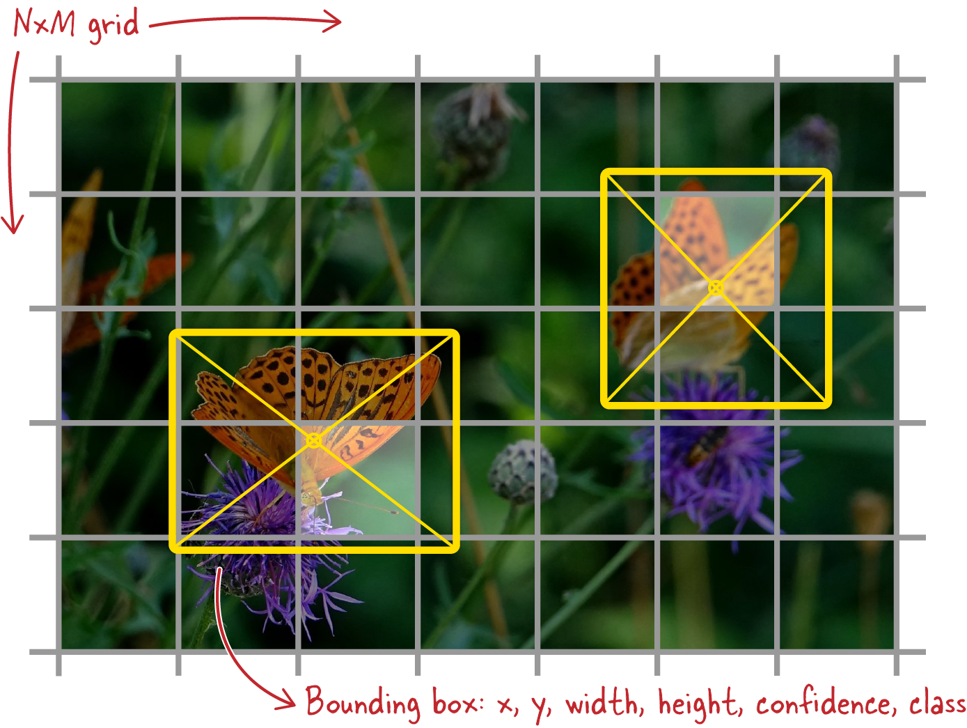
Figure 4-4. The YOLO grid. Each grid cell predicts a bounding box for an object whose center is somewhere in that cell. Image from Arthropods dataset.

Object detection head

Predicting a bounding box amounts to predicting six numbers: the four coordinates of the bounding box (in this case, the x and y coordinates of the center, and the width and height), a confidence factor which tells us if an object has been detected or not, and finally, the class of the object (for example, “butterfly”). The YOLO architecture does this directly on the last feature map, as generated by the convolutional backbone it is using.

In Figure 4-5, the x- and y-coordinate calculations use a hyperbolic tangent (tanh) activation so that the coordinates fall in the [–1, 1] range. They will be the coordinates of the center of the detection box, relative to the center of the grid cell they belong to.

Figure 4-5. A YOLO detection head predicts, for every grid cell, a bounding box (x, y, w, h), the confidence C of there being an object in this location, and the class of the object.

Width and height (w, h) calculations use a sigmoid activation so as to fall in the [0, 1] range. They will represent the size of the detection box relative to the entire image. This allows detection boxes to be bigger than the grid cell they originate in. The confidence factor, C, is also in the [0, 1] range. Finally, a softmax activation is used to predict the class of the detected object. The tanh and sigmoid functions are depicted in Figure 4-6.

Figure 4-6. The tanh and sigmoid activation functions. Tanh outputs values in the [–1, 1] range, while the sigmoid function outputs them in the [0, 1] range.

An interesting practical question is how to obtain a feature map of exactly the right dimensions. In the example from Figure 4-4, it must contain exactly 7 * 5 * (5 + 7) values. The 7 * 5 is because we chose a 7x5 YOLO grid. Then, for each grid cell, five values are needed to predict a box (x, y, w, h, C), and seven additional values are needed because, in this example, we want to classify arthropods into seven categories (Coleoptera, Aranea, Hemiptera, Diptera, Lepidoptera, Hymenoptera, Odonata).

If you control the convolutional stack, you could try to tune it to get exactly 7 * 5 * 12 (420) outputs at the end. However, there is an easier way: flatten whatever feature map the convolutional backbone is returning and feed it through a fully connected layer with exactly that number of outputs. You can then reshape the 420 values into a 7x5x12 grid, and apply the appropriate activations as in Figure 4-5. The authors of the YOLO paper argue that the fully connected layer actually adds to the accuracy of the system.

Loss function

In object detection, as in any supervised learning setting, the correct answers are provided in the training data: ground truth boxes and their classes. During training the network predicts detection boxes, and it has to take into account errors in the boxes’ locations and dimensions as well as misclassification errors, and also penalize detections of objects where there aren’t any. The first step, though, is to correctly pair ground truth boxes with predicted boxes so that they can be compared. In the YOLO architecture, if each grid cell predicts a single box, this is straightforward. A ground truth box and a predicted box are paired if they are centered in the same grid cell (see Figure 4-4 for easier understanding).

However in the YOLO architecture, the number of detection boxes per grid cell is a parameter. It can be more than one. If you look back to Figure 4-5, you can see that it’s easy enough for each grid cell to predict 10 or 15 (x, y, w, h, C) coordinates instead of 5 and generate 2 or 3 detection boxes instead of 1. But pairing these predictions with ground truth boxes requires more care. This is done by computing the intersection over union (IOU; see Figure 4-7) between all ground truth boxes and all predicted boxes within a grid cell, and selecting the pairings where the IOU is the highest.

Figure 4-7. The IOU metric.

To summarize, ground truth boxes are assigned to grid cells by their centers and to the prediction boxes within these grid cells by IOU.  With the pairings in place, we can now calculate the different parts of the loss:

Object presence loss

Each grid cell that has a ground truth box computes:

$L_{obj}=(1-C{)}^2$

Object absence loss

Each grid cell that does not have a ground truth box computes:

$L_{noobj}=(0-C{)}^2=C^2$

Object classification loss

Each grid cell that has a ground truth box computes:

$L_{class}=cros{s}_{-}entropy(p,\hat{p})$

where p̂ is the vector of predicted class probabilities and p is the one-hot-encoded target class.

Bounding box loss

Each predicted box/ground truth box pairing contributes (predicted coordinate marked with a hat, the other coordinate is the ground truth):

$L_{box}=(x-\hat{x}{)}^2+(y-\hat{y}{)}^2+{(\sqrt{w}-\sqrt{\hat{w}})}^2+(\sqrt{h}-\sqrt{\hat{h}}{)}^2$

Notice here that the difference in box sizes is computed on the square roots of the dimensions. This is to mitigate the effect of large boxes, which tend to overwhelm the loss.

Finally, all the loss contributions from the grid cells are added together, with weighting factors. A common problem in object detection losses is that small losses from numerous cells with no object in them end up overpowering the loss from a lone cell that predicts a useful box. Weighting different parts of the loss can alleviate this problem. The authors of the paper used the following empirical weights:

$\begin{array}{cccc}{\lambda }_{obj}=1& {\lambda }_{noobj}=0.5& {\lambda }_{class}=1& {\lambda }_{box}=5\end{array}$

YOLO limitations

The biggest limitation is that YOLO predicts a single class per grid cell and will not work well if multiple objects of different kinds are present in the same cell.

The second limitation is the grid itself: a fixed grid resolution imposes strong spatial constraints on what the model can do. YOLO models will typically not do well on collections of small objects, like a flock of birds, without careful tuning of the grid to the dataset.

Also, YOLO tends to localize objects with relatively low precision. The main reason for that is that it works on the last feature map from the convolutional stack, which is typically the one with the lowest spatial resolution and contains only coarse location signals.

Despite these limitations, the YOLO architecture is very simple to implement, especially with a single detection box per grid cell, which makes it a good choice when you want to experiment with your own code.

Note that it is not the case that every object is detected by looking at the information in a single grid cell. In a sufficiently deep convolutional neural network (CNN), every value in the last feature map, from which detection boxes are computed, depends on all the pixels of the original image.

If a higher accuracy is needed, you can step up to the next level: RetinaNet. It incorporates a number of ideas that improve upon the basic YOLO architecture, and is regarded, at the time of writing, as the state of the art of so-called single-shot detectors.

RetinaNet

RetinaNet, as compared to YOLOv1, has several innovations in its architecture and in the design of its losses. The neural network design includes feature pyramid networks which combine information extracted at multiple scales. The detection head predicts boxes starting from anchor boxes that change the bounding box representation to make training easier. Finally, the loss innovations include the focal loss, a loss specifically designed for detection problems, a smooth L1 loss for box regression, and non-max suppression. Let’s look at each of these in turn.

Feature pyramid networks

When an image is processed by a CNN, the initial convolutional layers pick up low-level details like edges and textures. Further layers combine them into features with more and more semantic value. At the same time, pooling layers in the network reduce the spatial resolution of the feature maps (see Figure 4-8).

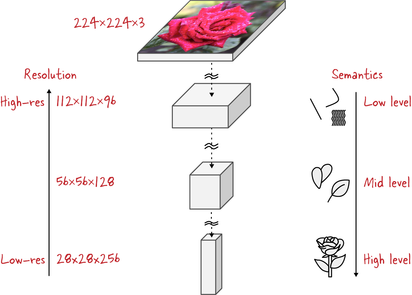
Figure 4-8. Feature maps at various stages of a CNN. As information progresses through the neural network, its spatial resolution decreases but its semantic content increases from low-level details to high-level objects.

The YOLO architecture only uses the last feature map for detection. It is able to correctly identify objects, but its localization accuracy is limited. Another idea would be to try and add a detection head at every stage. Unfortunately, in this approach, the heads working from the early feature maps would localize objects rather well but would have difficulty labeling them. At that early stage, the image has only gone through a couple of convolutional layers, which is not enough to classify it. Higher-level semantic information, like “this is a rose,” needs tens of convolutional layers to emerge.

Still, one popular detection architecture, called the single-shot detector (SSD), is based on this idea. The authors of the SSD paper made it work by connecting their multiple detection heads to multiple feature maps, all located toward the end of the convolutional stack.

What if we could combine all feature maps in a way that would surface both good spatial information and good semantic information at all scales? This can be done with a couple of additional layers forming a feature pyramid network. Figure 4-9 offers a schematic view of an FPN compared to the YOLO and SSD approaches, while Figure 4-10 presents the detailed design.

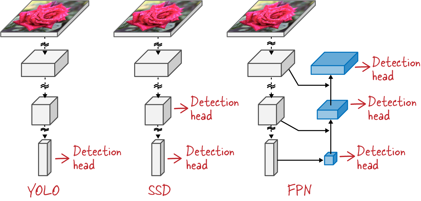
Figure 4-9. Comparison of YOLO, SSD, and FPN architectures and where, in the convolutional stack, they connect their detection head(s).

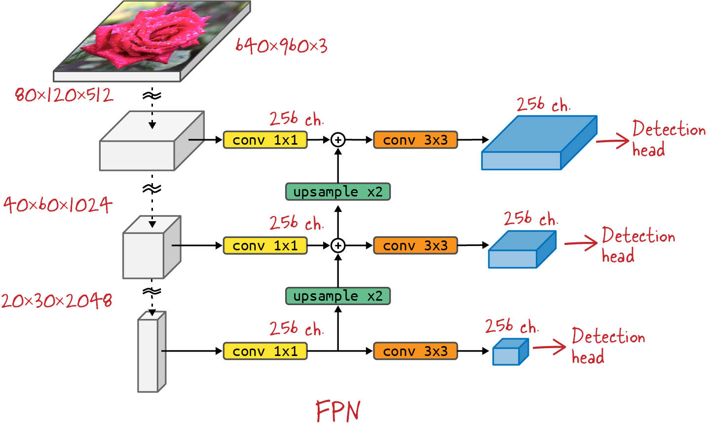
Figure 4-10. A feature pyramid network in detail. Feature maps are extracted from various stages of a convolutional backbone, and 1x1 convolutions squeeze every feature map to the same number of channels. Upsampling (nearest neighbor) then makes their spatial dimensions compatible so that they can be added up. The final 3x3 convolutions smooth out upsampling artifacts. Typically no activation functions are used in the FPN layers.

Here is what is happening in the FPN in Figure 4-10: in the downward path (convolutional backbone), convolutional layers gradually refine the semantic information in the feature maps, while pooling layers scale the feature maps down in their spatial dimensions (the x and y dimensions of the image). In the upward path, feature maps from the bottom layers containing good high-level semantic information get upsampled (using a simple nearest neighbor algorithm) so that they can be added, element-wise, to feature maps higher up in the stack. 1x1 convolutions are used in the lateral connections to bring all feature maps to the same channel depth and make the additions possible. The FPN paper, for example, uses 256 channels everywhere. The resulting feature maps now contain semantic information at all scales, which was the initial goal. They are further processed through a 3x3 convolution, mostly to smooth out the effects of the upsampling.

There are typically no nonlinearities in the FPN layers. The authors of the FPN paper found them to have little impact.

A detection head can now take the feature maps at each resolution and produce box detections and classifications. The detection head can itself have multiple designs, which we will cover in the next two sections. It will, however, be shared across all the feature maps at different scales. This is why it was important to bring all the feature maps to the same channel depth.

The nice thing about the FPN design is that it is independent of the underlying convolutional backbone. Any convolutional stack from Chapter 3 will do, as long as you can extract intermediate feature maps from it—typically four to six, at various scales. You can even use a pretrained backbone. Typical choices are ResNet or EfficientNet, and pretrained versions of them can be found in TensorFlow Hub.

There are multiple levels in a convolutional stack where features can be extracted and fed into the FPN. For each desired scale, many layers output feature maps of the same dimensions (see Figure 3-26 in the previous chapter). The best choice is the last feature map of a given block of layers outputting similarly sized features, just before a pooling layer halves the resolution again. This feature map is likely to contain the strongest semantic features.

It is also possible to extend an existing pretrained backbone with additional pooling and convolutional layers, for the sole purpose of feeding an FPN. These additional feature maps are typically small and therefore fast to process. They correspond to the lowest spatial resolution (see Figure 4-8) and can therefore improve the detection of large objects. The SSD paper actually used this trick, and RetinaNet does as well, as you will see in the architecture diagram later (Figure 4-15).

Anchor boxes

In the YOLO architecture, detection boxes are computed as deltas relative to a set of base boxes (Δx = x – x₀, Δy = y – y₀, Δw = w – w₀, Δh = h – h₀ are often referred to as “deltas” relative to some base box x₀, y₀, w₀, h₀ because of the Greek letter Δ, usually chosen to represent a ”difference”). In that case, the base boxes were a simple grid overlaid on the image (see Figure 4-4).

More recent architectures have expanded on this idea by explicitly defining a set of so-called “anchor boxes” with various aspect ratios and scales (examples in Figure 4-11). Predictions are again small variations of the size and position of the anchors. The goal is to help the neural network predict small values around zero rather than large ones. Indeed, neural networks are able to solve complex nonlinear problems because they use nonlinear activation functions between their layers. However, most activation functions (sigmoid, ReLU) exhibit a nonlinear behavior around zero only. That’s why neural networks are at their best when they predict small values around zero, and it’s why predicting detections as small deltas relative to anchor boxes is helpful. Of course, this only works if there are enough anchor boxes of various sizes and aspect ratios that any object detection box can be paired (by max IOU) with an anchor box of closely matching position and dimensions.

Figure 4-11. Examples of anchor boxes of various sizes and aspect ratios used to predict detection boxes. Image from Arthropods dataset.

We will describe in detail the approach taken in the RetinaNet architecture, as an example. RetinaNet uses nine different anchor types with:

• Three different aspect ratios: 2:1, 1:1, 1:2

• Three different sizes: 2⁰, 2^⅓, 2^⅔ (≃ 1, 1.3, 1.6)

They are depicted in Figure 4-12.

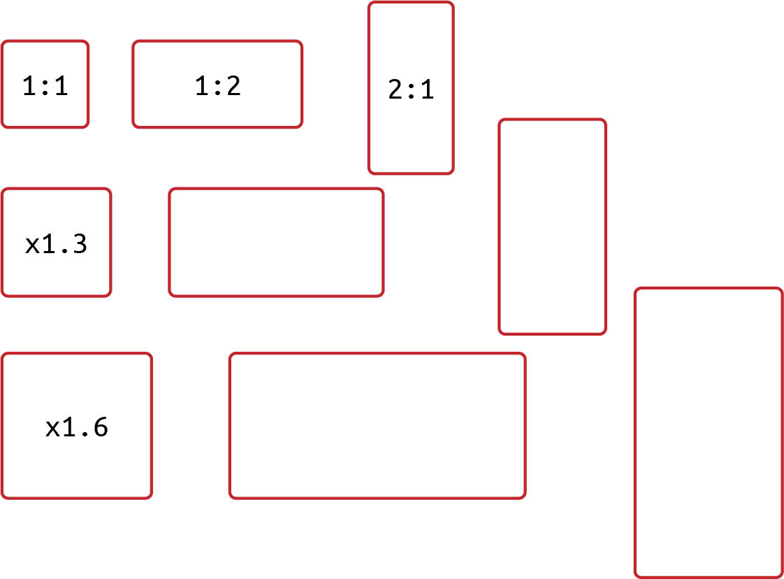
Figure 4-12. The nine different anchor types used in RetinaNet. Three aspect ratios and three different sizes.

Anchors, along with the feature maps computed by an FPN, are the inputs from which detections are computed in RetinaNet. The sequence of operations is as follows:

• The FPN reduces the input image into five feature maps (see Figure 4-10).

• Each feature map is used to predict bounding boxes relative to anchors at regularly spaced locations throughout the image. For example, a feature map of size 4x6 with 256 channels will use 24 (4 * 6) anchor locations in the image (see Figure 4-13).

• The detection head uses multiple convolutional layers to convert the 256-channel feature map into exactly 9 * 4 = 36 channels, yielding 9 detection boxes per location. The four numbers per detection box represent the deltas relative to the center (x, y), the width, and the height of the anchor. The precise sequence of the layers that compute detections from the feature maps is shown in Figure 4-15.

• Finally, each feature map from the FPN, since it corresponds to a different scale in the image, will use different scales of anchor boxes.

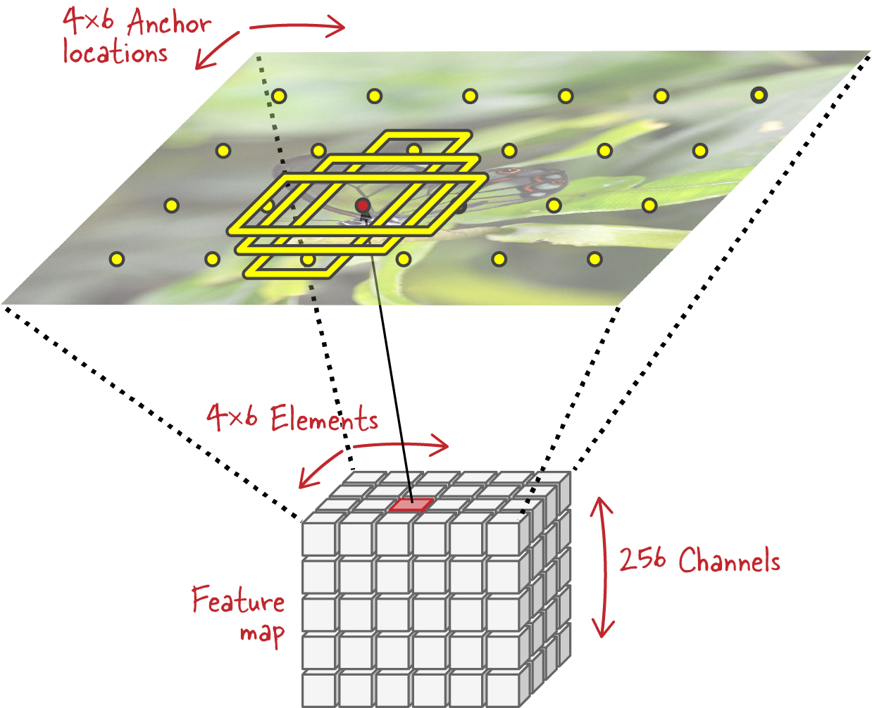
Figure 4-13. Conceptual view of the RetinaNet detection head. Each spatial location in a feature map corresponds to a series of anchors in the image, all centered at the same point. For clarity, only three such anchors are shown in the illustration, but RetinaNet would have nine at every location.

The anchors themselves are spaced regularly across the input image and sized appropriately for each level of the feature pyramid. For example in RetinaNet, the following parameters are used:

• The feature pyramid has five levels corresponding to scales P₃, P₄, P₅, P₆, and P₇ in the backbone. Scale P_n represents a feature map 2ⁿ times smaller in width and height than the input image (see the complete RetinaNet view in Figure 4-15).

• Anchor base sizes are 32x32, 64x64, 128x128, 256x256, 512x512 pixels, at each feature pyramid level respectively (= 4 * 2ⁿ, if n is the scale level).

• Anchor boxes are considered for every spatial location of every feature map in the feature pyramid, which means that the boxes are spaced every 8, 16, 32, 64, or 128 pixels across the input image at each feature pyramid level, respectively (= 2ⁿ, if n is the scale level).

The smallest anchor box is therefore 32x32 pixels while the largest one is 812x1,624 pixels.

Note

The anchor box settings must be tuned for every dataset so that they correspond to the detection box characteristics actually found in the training data. This is typically done by resizing input images rather than changing the anchor box generation parameters. However, on specific datasets with many small detections, or, on the contrary, mostly large objects, it can be necessary to tune the anchor box generation parameters directly.

The last step is to compute a detection loss. For that, predicted detection boxes must be paired with ground truth boxes so that detection errors can be evaluated.

The assignment of ground truth boxes to anchor boxes is based on the IOU metric computed between each set of boxes in one input image. All pairwise IOUs are computed and are arranged in a matrix with N rows and M columns, N being the number of ground truth boxes and M the number of anchor boxes. The matrix is then analyzed by columns (see Figure 4-14):

• An anchor is assigned to the ground truth box that has the largest IOU in its column, provided it is more than 0.5.

• An anchor box that has no IOU greater than 0.4 in its column is assigned to detect nothing (i.e., the background of the image).

• Any unassigned anchor at this point is marked to be ignored during training. Those are anchors with IOUs in the intermediate regions between 0.4 and 0.5.

Now that every ground truth box is paired with exactly one anchor box, it is possible to compute box predictions, classifications, and the corresponding losses.

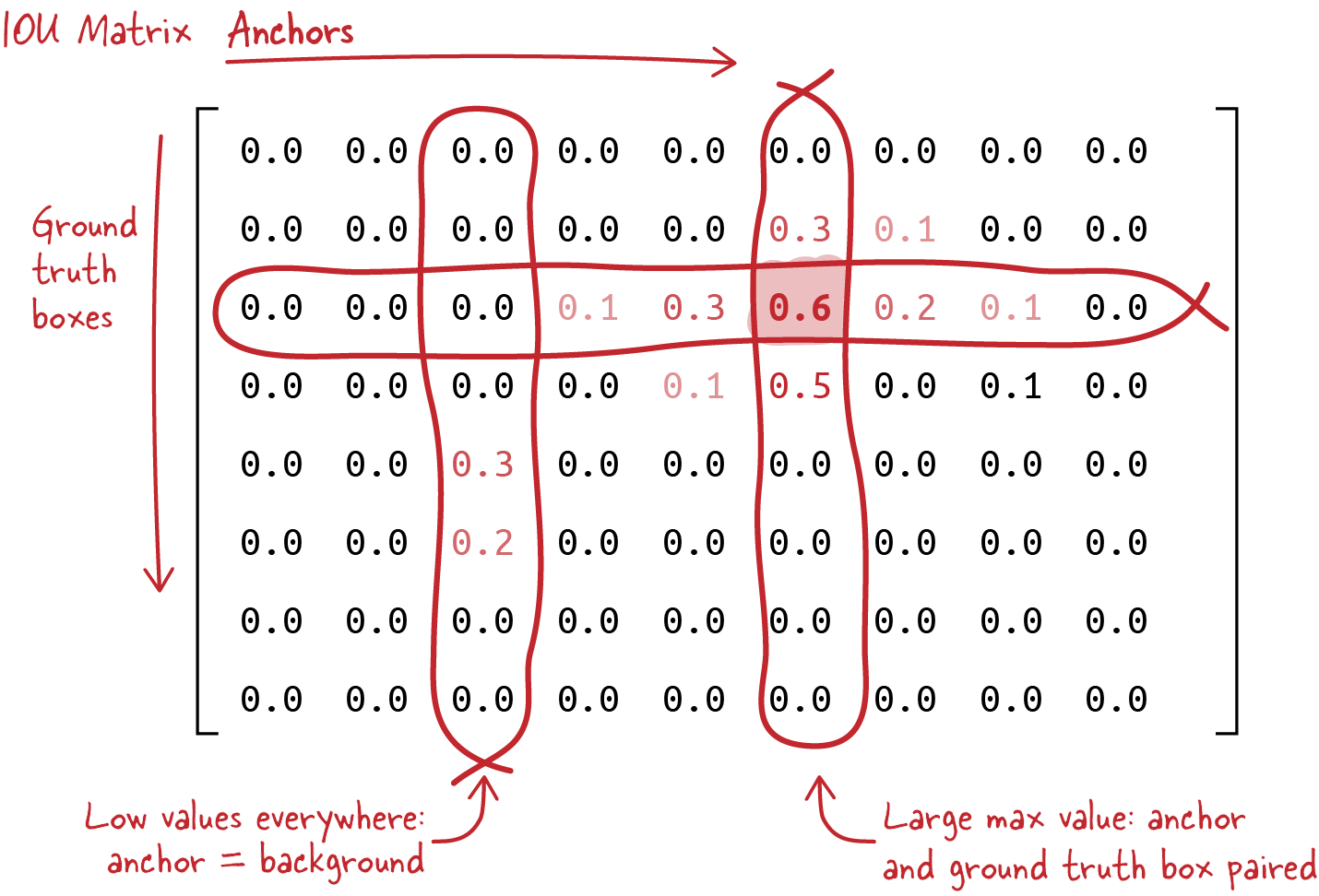
Figure 4-14. The pairwise IOU metric is computed between all ground truth boxes and all anchor boxes to determine their pairings. Anchors without a meaningful intersection with a ground truth box are deemed “background” and trained to detect nothing.

Architecture

The detection and classification heads transform the feature maps from the FPN into class predictions and bounding box deltas. Feature maps are three-dimensional. Two of their dimensions correspond to the x and y dimensions of the image and are called spatial dimensions; the third dimension is their number of channels.

In RetinaNet, for every spatial location in every feature map, the following parameters are predicted (with K = the number of classes and B = the number of anchor box types, so in our case B=9):

• The class prediction head predicts B * K probabilities, one set of probabilities for every anchor type. This in effect predicts one class for every anchor.

• The detection head predicts B * 4 = 36 box deltas Δx, Δy, Δw, Δh. Bounding boxes are still parameterized by their center (x, y) as well as their width and height (w, h).

Both heads share a similar design, although with different weights, and the weights are shared across all scales in the feature pyramid.

Figure 4-15 represents a complete view of the RetinaNet architecture. It uses a ResNet50 (or other) backbone. The FPN extracts features from backbone levels P₃ though P_7, where P_n is the level where the feature map is reduced by a factor of 2ⁿ in its width and height compared to the original image. The FPN part is described in detail in Figure 4-10. Every feature map from the FPN is fed through both a classification and a box regression head.

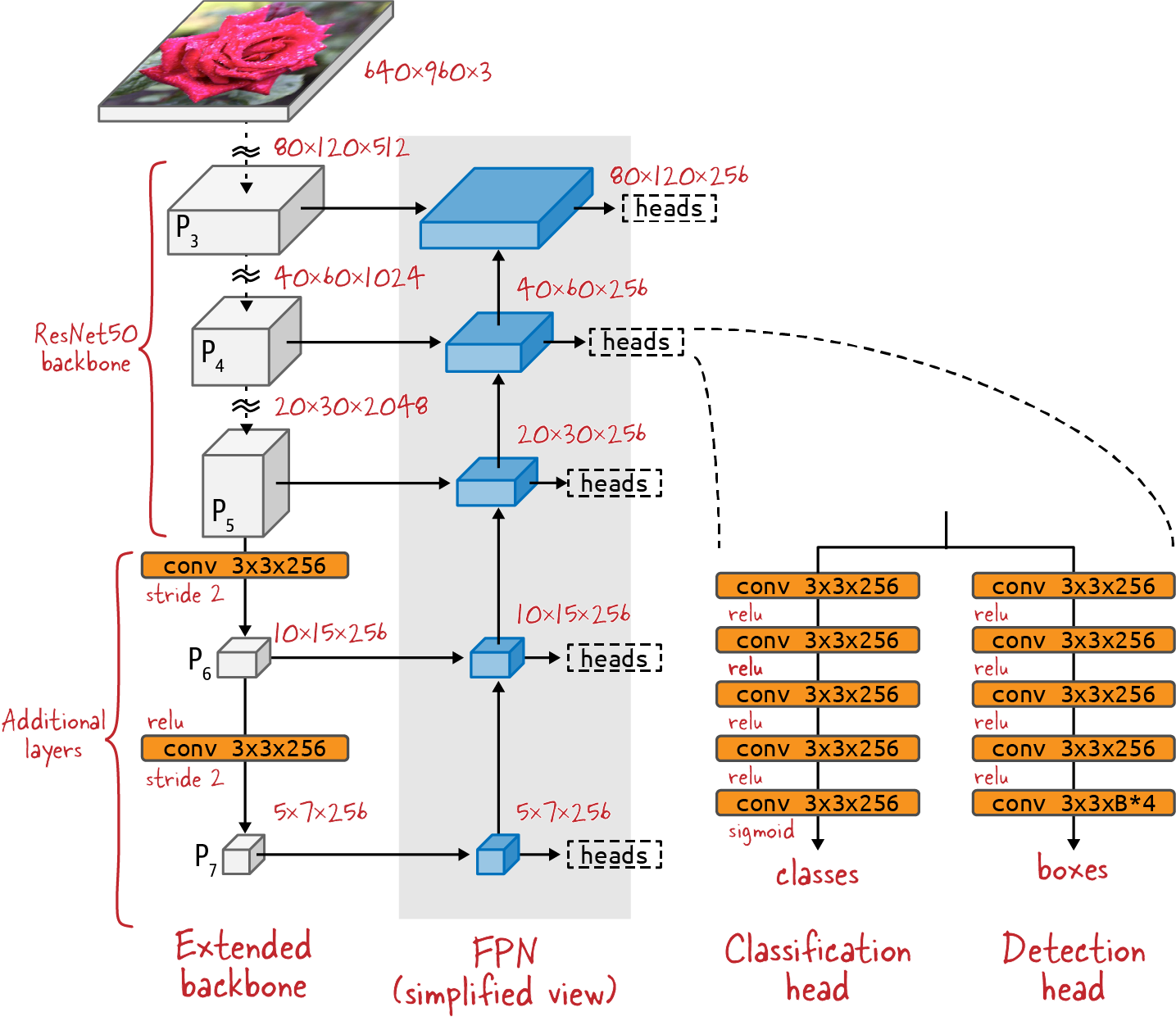
Figure 4-15. Complete view of the RetinaNet architecture. K is the number of target classes. B is the number of anchor boxes at each position, which is nine in RetinaNet.

The RetinaNet FPN taps into the three last scale levels available from the backbone. The backbone is extended with 2 additional layers using a stride of 2 to provide 2 additional scale levels to the FPN. This architectural choice allows RetinaNet to avoid processing very large feature maps, which would be time-consuming. The addition of the last two coarse scale levels also improves the detection of very large objects.

The classification and box regression heads themselves are made from a simple sequence of 3x3 convolutions. The classification head is designed to predict K binary classifications for every anchor, which is why it ends on a sigmoid activation. It looks like we are allowing multiple labels to be predicted for every anchor, but actually the goal is to allow the classification head to output all zeros, which will represent the “background class” corresponding to no detections. A more typical activation for classification would be softmax, but the softmax function cannot output all zeros.

The box regression ends with no activation function. It is computing the differences between the center coordinates (x, y), width, and height of the anchor box and detection box. Some care must be taken to allow the regressor to work in the [–1, 1] range at all levels in the feature pyramid. The following formulas are used to achieve that:

• X_pixels = X × U × W_A + X_A

• Y_pixels = Y × U × H_A + Y_A

• W_pixels = W_A × e^{W × V}

• H_pixels = H_A × e^{H × V}

In these formulas, X_A, Y_A, W_A, and H_A are the coordinates of an anchor box (center coordinates, width, height), while X, Y, W, and H are the predicted coordinates relative to the anchor box (deltas). X_pixels, Y_pixels, W_pixels, and H_pixels are the actual coordinates, in pixels, of the predicted box (center and size). U and V are modulating factors that correspond to the expected variance of the deltas relative to the anchor box. Typical values are U=0.1 for coordinates, and V=0.2 for sizes. You can verify that values in the [–1, 1] range for predictions result in predicted boxes that fall within ±10% of the position of the anchor and within ±20% of its size.

Focal loss (for classification)

How many anchor boxes are considered for one input image? Looking back at Figure 4-15, with an example input image of 640x960 pixels, the five different feature maps in the feature pyramid represent 80 * 120 + 40 * 60 + 20 * 30+ 10 * 15 + 5 * 7 = 12,785 locations in the input image. With 9 anchor boxes per location, that’s slightly over 100K anchor boxes.

This means that 100K predicted boxes will be generated for every input image. In comparison, there are 0 to 20 ground truth boxes per image in a typical application. The problem this creates in detection models is that the loss corresponding to background boxes (boxes assigned to detect nothing) can overwhelm the loss corresponding to useful detections in the total loss. This happens even if background detections are already well trained and produce a small loss. This small value multiplied by 100K can still be orders of magnitude larger than the detection loss for actual detections. The end result is a model that cannot be trained.

The RetinaNet paper suggested an elegant solution to this problem: the authors tweaked the loss function to produce much smaller values on empty backgrounds. They call this the focal loss. Here are the details.

We have already seen that RetinaNet uses a sigmoid activation to generate class probabilities. The output is a series of binary classifications, one for every class. A probability of 0 for every class means “background”; i.e., nothing to detect here. The classification loss used is the binary cross-entropy. For every class, it is computed from the actual binary class label y (0 or 1) and the predicted probability for the class p using the following formula:

$CE(y,p)=-y\cdot \log \left(p\right)-(1-y)\cdot \log (1-p)$

The focal loss is the same formula with a small modification:

$FL(y,p)=-y\cdot (1-p{)}^{\gamma }\cdot \log \left(p\right)-(1-y)\cdot p^{\gamma }\cdot \log (1-p)$

For γ=0 this is exactly the binary cross-entropy, but for higher values of γ the behavior is slightly different. To simplify, let’s only consider the case of background boxes that do not belong to any class (i.e., where y=0 for all classes):

$F{L}_{bkg}\left(p\right)=-p^{\gamma }\cdot \log (1-p)$

And let’s plot the values of the focal loss for various values of p and γ (Figure 4-16).

As you can see in the figure, with γ=2, which was found to be an adequate value, the focal loss is much smaller than the regular cross-entropy loss, especially for small values of p. For background boxes, where there is nothing to detect, the network will quickly learn to produce small class probabilities p across all classes. With the cross-entropy loss, these boxes, even well classified as “background” with p=0.1 for example, would still be contributing a significant amount: CE(0.1) = 0.05. The focal loss is 100 times less: FL(0.1) = 0.0005.

With the focal loss, it becomes possible to add the losses from all anchor boxes—all 100K of them—and not worry about the total loss being overwhelmed by thousands of small losses from easy-to-classify background boxes.

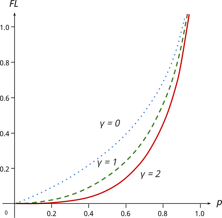
Figure 4-16. Focal loss for various values of γ. For γ=0, this is the cross-entropy loss. For higher values of γ, the focal loss greatly de-emphasizes easy-to-classify background regions where p is close to 0 for every class.

Smooth L1 loss (for box regression)

Detection boxes are computed by a regression. For regressions, the two most common losses are L1 and L2, also called absolute loss and squared loss. Their formulas are (computed between a target value a and the predicted value â):

$\begin{array}{l}L1(a,\hat{a})=|a-\hat{a}|\\ L2(a,\hat{a})=(a-\hat{a}{)}^2\end{array}$

The problem with the L1 loss is that its gradient is the same everywhere, which is not great for learning. The L2 loss is therefore preferred for regressions—but it suffers from a different problem. In the L2 loss, differences between the predicted and target values are squared, which means that the loss tends to get very large as the prediction and the target grow apart. This becomes problematic if you have some outliers, like a couple of bad points in the data (for example, a target box with the wrong size). The result will be that the network will try to fit the bad data point at the expense of everything else, which is not good either.

A good compromise between the two is the Huber loss, or smooth L1 loss (see Figure 4-17). It behaves like the L2 loss for small values and like the L1 loss for large values. Close to zero, it has the nice property that its gradient is larger when the differences are larger, and therefore it pushes the network to learn more where it is making the biggest mistakes. For large values, it becomes linear instead of quadratic and avoids being thrown off by a couple of bad target values. Its formula is:

$\begin{array}{cc}\hfill L_{\delta }(a-\hat{a})={\displaystyle \frac{1}{2}}(a-\hat{a}{)}^2& \text{for}|a-\hat{a}|\le \delta \\ \hfill \begin{array}{c}{L}_{\delta }=\delta \left(|a-\hat{a}|-{\displaystyle \frac{1}{2}}\delta \right)\end{array}& \text{otherwise}\end{array}$

Where δ is an adjustable parameter. δ is the value around which the behavior switches from quadratic to linear. Another formula can be used to avoid the piecewise definition:

$L_{\delta }(a-\hat{a})={\delta }^2\left(\sqrt{1+({\displaystyle \frac{a-\hat{a}}{\delta }}{)}^2-1}\right)$

This alternate form does not give the exact same values as the standard Huber loss, but it has the same behavior: quadratic for small values, linear for large ones. In practice, either form will work well in RetinaNet, with δ=1.

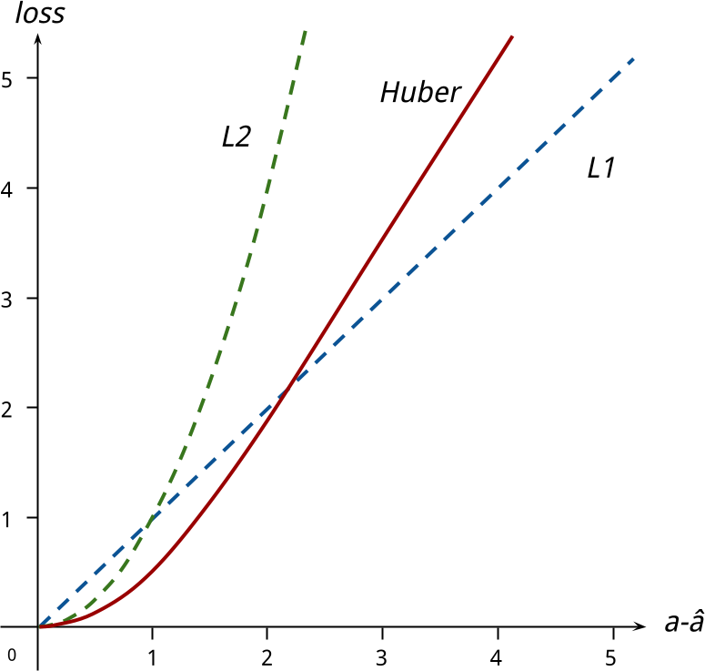
Figure 4-17. L1, L2, and Huber losses for regression. The desirable behaviors are quadratic for small values and linear for large ones. The Huber loss has both.

Non-maximum suppression

A detection network using numerous anchor boxes, such as RetinaNet, usually produces multiple candidate detections for every target box. We need an algorithm to select a single detection box for every detected object.

Non-maximum suppression (NMS) takes box overlap (IOU) and class confidence into account to select the most representative box for a given object (Figure 4-18).

Figure 4-18. On the left: multiple detections for the same object. On the right: a single box remaining after non-max suppression. Image from Arthropods dataset.

The algorithm uses a simple “greedy” approach: for every class, it considers the overlap (IOU) between all the predicted boxes. If two boxes overlap more than a given value A (IOU > A), it keeps the one with the highest class confidence. In Python-like pseudocode, for one given class:

def NMS(boxes, class_confidence):
    result_boxes = []
    for b1 in boxes:
        discard = False
        for b2 in boxes:
            if IOU(b1, b2) > A:
                if class_confidence[b2] > class_confidence[b1]:
                    discard = True
        if not discard:
            result_boxes.append(b1)
    return result_boxes

NMS works quite well in practice but it can have some unwanted side effects. Notice that the algorithm relies on a single threshold value (A). Changing this value changes the box filtering, especially for adjacent or overlapping objects in the original image. Take a look at the example in Figure 4-19. If the threshold is set at A=0.4, then the two boxes detected in the figure will be regarded as “overlapping” for the same class and the one with the lowest class confidence (the one on the left) will be discarded. That is obviously wrong. There are two butterflies to detect in this image and, before NMS, both were detected with a high confidence.

Figure 4-19. Objects close to each other create a problem for the non-max suppression algorithm. If the NMS threshold is 0.4, the box detected on the left will be discarded, which is wrong. Image from Arthropods dataset.

Pushing the threshold value higher will help, but if it’s too high the algorithm will fail to merge boxes that correspond to the same object. The usual value for this threshold is A=0.5, but it still causes objects that are close together to be detected as one.

A slight variation on the basic NMS algorithm is called Soft-NMS. Instead of removing non-maximum overlapping boxes altogether, it lowers their confidence score by the factor:

$\mathit{exp}(-{\displaystyle \frac{IO{U}^2}{\sigma }})$

with σ being an adjustment factor that tunes the strength of the Soft-NMS algorithm. A typical value is σ=0.5. The algorithm is applied by considering the box with the highest confidence score for a given class (the max box), and decreasing the scores for all other boxes by this factor. The max box is then put aside and the operation is repeated on the remaining boxes until none remain.

For nonoverlapping boxes (IOU=0), this factor is 1. The confidence factors of boxes that do not overlap the max box are thus not affected. The factor gradually, but continuously, decreases as boxes overlap more with the max box. Highly overlapping boxes (IOU=0.9) get their confidence factor decreased by a lot (×0.2), which is the expected behavior because they are redundant with the max box and we want to get rid of them.

Since the Soft-NMS algorithm does not discard any boxes, a second threshold, based on the class confidence, is used to actually prune the list of detections.

The effect of Soft-NMS on the example from Figure 4-19 is shown in Figure 4-20.

Figure 4-20. Objects close to each other as handled by Soft-NMS. The detection box on the left is not deleted, but its confidence factor is reduced from 78% to 55%. Image from Arthropods dataset.

Note

In TensorFlow, both styles of non-max suppression are available. Standard NMS is called tf.image.non_max_suppression, while Soft-NMS is called tf.image.non_max_suppression_with_scores.

Other considerations

In order to reduce the amount of data needed, it is customary to use a pretrained backbone.

Classification datasets are much easier to put together than object detection datasets. That’s why readily available classification datasets are typically much larger than object detection datasets. Using a pretrained backbone from a classifier allows you to combine a generic large classification dataset with a task-specific object detection dataset and obtain a better object detector.

The pretraining is done on a classification task. Then the classification head is removed and the FPN and detection heads are added, initialized at random. The actual object detection training is performed with all weights trainable, which means that the backbone will be fine-tuned while the FPN and detection head train from scratch.

Since detection datasets tend to be smaller, data augmentation (which we will cover in more detail in Chapter 6) plays an important part in training. The basic data augmentation technique is to cut fixed-sized crops out of the training images at random, and at random zoom factors (see Figure 4-21). With target bounding boxes adjusted appropriately, this allows you to train the network with the same object at different locations in the image, at different scales and with different parts of the background visible.

Figure 4-21. Data augmentation for detection training. Fixed-size images are cut at random from each training image, potentially at different zoom factors. Target box coordinates are recomputed relative to the new boundaries. This provides more training images and more object locations from the same initial training data. Image from Arthropods dataset.

A practical advantage of this technique is that it also provides fixed-sized training images to the neural network. You can train directly on a training dataset made up of images of different sizes and aspect ratios. The data augmentation takes care of getting all the images to the same size.

Finally, what drives training and hyperparameter tuning are metrics. Object detection problems have been the subject of multiple large-scale contests where detection metrics have been carefully standardized; this topic is covered in detail in “Metrics for Object Detection” in Chapter 8.

Now that we have looked at object detection, let’s turn our attention to another class of problems: image segmentation.

Segmentation

Object detection finds bounding boxes around objects and classifies them. Instance segmentation adds, for every detected object, a pixel mask that gives the shape of the object. Semantic segmentation, on the other hand, does not detect specific instances of objects but classifies every pixel of the image into a category like “road,” “sky,” or “people.”

Mask R-CNN and Instance Segmentation

YOLO and RetinaNet, which we covered in the previous section, are examples of single-shot detectors. An image traverses them only once to produce detections. Another approach is to use a first neural network to suggest potential locations for objects to be detected, then use a second network to classify and fine-tune the locations of these proposals. These architectures are called region proposal networks (RPNs).

They tend to be more complex and therefore slower than single-shot detectors, but are also more accurate. There is a long list of RPN variants, all based on the original “regions with CNN features” idea: R-CNN, Fast R-CNN, Faster R-CNN, and more. The state of the art, at the time of writing, is Mask R-CNN, and that’s the architecture we are going to dive into next.

The main reason why it is important to be aware of architectures like Mask R-CNN is not their marginally superior accuracy, but the fact that they can be extended to perform instance segmentation tasks. In addition to predicting a bounding box around detected objects, they can be trained to predict their outline—i.e., find every pixel belonging to each detected object (Figure 4-22). Of course, training them remains a supervised training task and the training data will have to contain ground truth segmentation masks for all objects. Unfortunately, masks are more time-consuming to generate by hand than bounding boxes and therefore instance segmentation datasets are harder to find than simple object detection datasets.

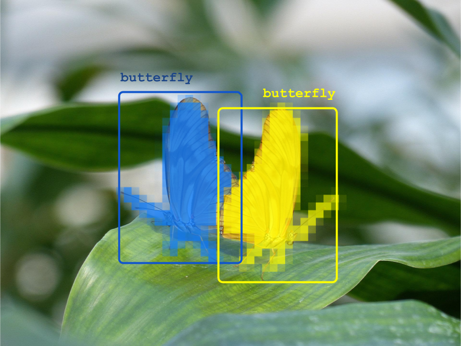
Figure 4-22. Instance segmentation involves detecting objects and finding all the pixels that belong to each object. The objects in the images are shaded with a pixel mask. Image from Arthropods dataset.

Let’s look at RPNs in detail, first analyzing how they perform classic object detection, then how to extend them for instance segmentation.

Region proposal networks

An RPN is a simplified single-shot detection network that only cares about two classes: objects and background. An “object” is anything labeled as such in the dataset (any class), and “background” is the designated class for a box that does not contain an object.

An RPN can use an architecture similar to the RetinaNet setup we looked at earlier: a convolutional backbone, a feature pyramid network, a set of anchor boxes, and two heads. One head is for predicting boxes and the other is for classifying them as object or background (we are not predicting segmentation masks yet).

The RPN has its own loss function, computed from a slightly modified training dataset: the class of any ground truth object is replaced with a single class “object.” The loss function used for boxes is, as in RetinaNet, the Huber loss. For classes, since this is a binary classification, binary cross-entropy is the best choice.

Boxes predicted by the RPN then undergo non-max suppression. The top N boxes, sorted by their probability of being an “object,” are regarded as box proposals or regions of interest (ROIs) for the next stage. N is usually around one thousand, but if fast inference is important, it can be as little as 50. ROIs can also be filtered by a minimal “object” score or a minimal size. In the TensorFlow Model Garden implementation, these thresholds are available even if they are set to zero by default. Bad ROIs can still be classified as “background” and rejected by the next stage, so letting them through at the RPN level is not a big problem.

One important practical consideration is that the RPN can be simple and fast if needed (see the example in Figure 4-23). It can use the output of the backbone directly, instead of using an FPN, and its classification and detection heads can use fewer convolutional layers. The goal is only to compute approximate ROIs around likely objects. They will be refined and classified in the next step.

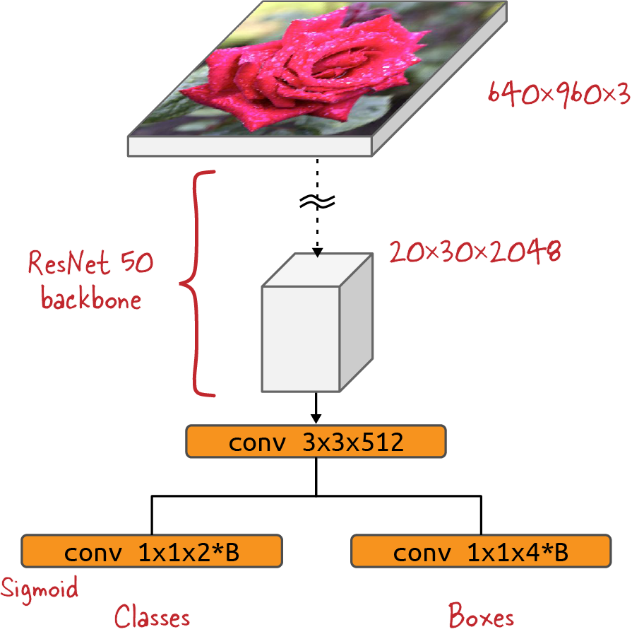
Figure 4-23. A simple region proposal network. The output from the convolutional backbone is fed through a two-class classification head (object or background) and a box regression head. B is the number of anchor boxes per location (typically three). An FPN can be used as well.

For example, the Mask R-CNN implementation in the TensorFlow Model Garden uses an FPN in its RPN but uses only three anchors per location, with aspect ratios of 0.5, 1.0, and 2.0, instead of the nine anchors per location used by RetinaNet.

R-CNN

We now have a set of proposed regions of interest. What next?

Conceptually, the R-CNN idea (Figure 4-24) is to crop the images along the ROIs and run the cropped images through the backbone again, this time with a full classification head attached to classify the objects (in our example, into “butterfly,” “spider,” etc.).

Figure 4-24. Conceptual view of an R-CNN. Images go through the backbone twice: the first time to generate regions of interest and the second time to classify the contents of these ROIs. Image from Arthropods dataset.

In practice, however, this is too slow. The RPN can generate somewhere in the region of 50 to 2,000 proposed ROIs, and running them all through the backbone again would be a lot of work. Instead of cropping the image, the smarter thing to do is to crop the feature map directly, then run prediction heads on the result, as depicted in Figure 4-25.

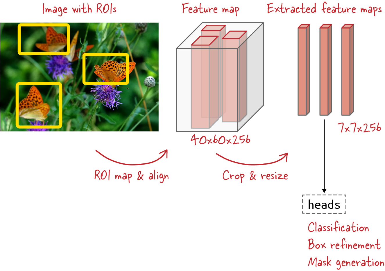
Figure 4-25. A faster R-CNN or Mask R-CNN design. As previously, the backbone generates a feature map and the RPN predicts regions of interest from it (only the result is shown). Then the ROIs are mapped back onto the feature map, and features are extracted and sent to the prediction heads for classification and more. Image from Arthropods dataset.

This is slightly more complex when an FPN is used. The feature extraction is still performed on a given feature map, but in a FPN there are several feature maps to choose from. A ROI therefore must first be assigned to the most relevant FPN level. The assignment is usually done using this formula:

$n=floor(n_0+{\mathit{log}}_2(\sqrt{wh}/224))$

where w and h are the width and height of the ROI, and n₀ is the FPN level where typical anchor box sizes are closest to 224. Here, floor stands for rounding down to the most negative number. For example, here are the typical Mask R-CNN settings:

• Five FPN levels, P₂, P₃, P₄, P₅, and P₆ (reminder: level P_n represents a feature map 2ⁿ times smaller in width and height than the input image)

• Anchor box sizes of 32x32, 64x64, 128x128, 256x256, and 512x512 on their respective levels (same as in RetinaNet)

• n₀ = 4

With these settings, we can verify that (for example) an ROI of 80x160 pixels would get assigned to level P₃ and an ROI of 200x300 to level P₄, which makes sense.

ROI resampling (ROI alignment)

Special care is needed when extracting the feature maps corresponding to the ROIs. The feature maps must be extracted and resampled correctly. The Mask R-CNN paper’s authors discovered that any rounding error made during this process adversely affects detection performance. They called their precise resampling method ROI alignment.

For example, let’s take an ROI of 200x300 pixels. It would be assigned to FPN level P₄, where its size relative to the P₄ feature map becomes (200 / 2⁴, 300 / 2⁴) = (12.5, 18.75). These coordinates should not be rounded. The same applies to its position.

The features contained in this 12.5x18.75 region of the P₄ feature map must then be sampled and aggregated (using either max pooling or average pooling) into a new feature map, typically of size 7x7. This is a well-known mathematical operation called bilinear interpolation, and we won’t dwell on it here. The important point to remember is that cutting corners here degrades performance.

Class and bounding box predictions

The rest of the model is pretty standard. The extracted features go through multiple prediction heads in parallel—in this case:

• A classification head to assign a class to each object suggested by the RPN, or classify it as background

• A box refinement head that further adjusts the bounding box

To compute detection and classification losses, the same target box assignment algorithm is used as in RetinaNet, described in the previous section. The box loss is also the same (Huber loss). The classification head uses a softmax activation with a special class added for “background.” In RetinaNet it was a series of binary classifications. Both work, and this implementation detail is not important. The total training loss is the sum of the final box and classification losses as well as the box and classification losses from the RPN.

The exact design of the class and detection heads is given later, in Figure 4-30. They are also very similar to what was used in RetinaNet: a straight sequence of layers, shared between all levels of the FPN.

Mask R-CNN adds a third prediction head for classifying individual pixels of objects. The result is a pixel mask depicting the silhouette of the object (see Figure 4-19). It can be used if the training dataset contains corresponding target masks. Before we explain how it works, however, we need to introduce a new kind of convolution, one capable of creating pictures rather than filtering and distilling them: transposed convolutions.

Transposed convolutions

Transposed convolutions, sometimes also called deconvolutions, perform a learnable upsampling operation. Regular upsampling algorithms like nearest neighbor upsampling or bilinear interpolation are fixed operations. Transposed convolutions, on the other hand, involve learnable weights.

Note

The name “transposed convolution” comes from the fact that in the matrix representation of a convolutional layer, which we are not covering in this book, the transposed convolution is performed using the same convolutional matrix as an ordinary convolution, but transposed.

The transposed convolution pictured in Figure 4-26 has a single input and a single output channel. The best way to understand what it does is to imagine that it is painting with a brush on an output canvas. The brush is a 3x3 filter. Every value of the input image is projected through the filter on the output. Mathematically, every element of the 3x3 filter is multiplied by the input value and the result is added to whatever is already on the output canvas. The operation is then repeated at the next position: in the input we move by 1, and in the output we move with a configurable stride (2 in this example). Any stride larger than 1 results in an upsampling operation. The most frequent settings are stride 2 with a 2x2 filter or stride 3 with a 3x3 filter.

If the input is a feature map with multiple channels, the same operation is applied to each channel independently, with a new filter each time; then all the outputs are added element by element, resulting in a single output channel.

It is of course possible to repeat this operation multiple times on the same feature map, with a new set of filters each time, which results in a feature map with multiple channels.

In the end, for a multichannel input and a multichannel output, the weights matrix of a transposed convolution will have the shape shown in Figure 4-27. This is, by the way, the same shape as a regular convolutional layer.

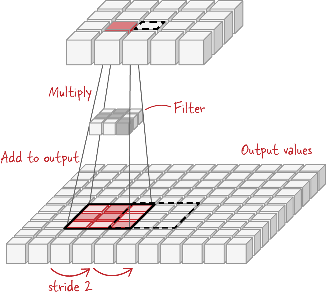
Figure 4-26. Transposed convolution. Each pixel of the original image (top) multiplies a 3x3 filter, and the result is added to the output. In a transposed convolution of stride 2, the output window moves by a step of 2 for every input pixel, creating a larger image (shifted output window pictured with a dashed outline).

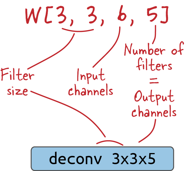
Figure 4-27. The weights matrix of a transposed convolutional layer, sometimes also called a “deconvolution.” At the bottom is the schematic notation of deconvolutional layers that will be used for the models in this chapter.

Up-Convolution

Transposed convolutions are widely used in neural networks that generate images: autoencoders, generative adversarial networks (GANs), and so on. However, they have also been criticized for introducing “checkerboard” artifacts into the generated images (Odena et al., 2016), especially when their stride and filter size are not multiples of each other (Figure 4-28).

Figure 4-28. Transposed convolutions versus up-convolutions when used in a GAN. When transposed convolutions are used, an unwanted checkerboard pattern can appear (top row). This does not happen with up-convolutions. Image from Odena et al., 2016.

Odena et al. suggest using a simple nearest neighbour resampling followed by a regular convolution, a combination called “up-convolution” (Figure 4-29), instead of transposed convolutions. Interestingly, as you may recall from “Feature pyramid networks”, this is exactly how upsampling was handled there.

Figure 4-29. This is also a learnable upsampling operation. An “up-convolution” is a simple nearest neighbor upsampling operation followed by an ordinary convolutional layer.

Instance segmentation

Let’s get back to Mask R-CNN, and its third prediction head that classifies individual pixels of objects. The output is a pixel mask outlining the silhouette of the object (see Figure 4-22).

Mask R-CNN and other RPNs work on a single ROI at a time, with a fairly high probability that this ROI is actually interesting, so they can do more work per ROI and with a higher precision. Instance segmentation is one such task.

The instance segmentation head uses transposed convolution layers to upsample the feature map into a black-and-white image that is trained to match the silhouette of the detected object.

Figure 4-30 shows the complete Mask R-CNN architecture.

Figure 4-30. The Mask R-CNN architecture. N is the number of ROIs proposed by the RPN, and K is the number of classes; “deconv” denotes a transposed convolutional layer, which upsamples the feature maps to predict an object mask.

Notice that the mask head produces one mask per class. This seems to be redundant since there is a separate classification head. Why predict K masks for one object? In reality, this design choice increases the segmentation accuracy because it allows the segmentation head to learn class-specific hints about objects.

Another implementation detail is that the resampling and alignment of the feature maps to the ROIs is actually performed twice: once with a 7x7x256 output for the classification and detection head, and again with different settings (resampling to 14x14x256) specifically for the mask head to give it more detail to work with.

The segmentation loss is a simple pixel-by-pixel binary cross-entropy loss, applied once the predicted mask has been rescaled and upsampled to the same coordinates as the ground truth mask. Note that only the mask predicted for the predicted class is taken into account in the loss calculation. Other masks computed for the wrong classes are ignored.

We now have a complete picture of how Mask R-CNN works. One thing to notice is that with all the improvements added to the R-CNN family of detectors, Mask R-CNN is now a “two-pass” detector in name only. The input image effectively goes through the system only once. The architecture is still slower than RetinaNet but achieves a slightly higher detection accuracy and adds instance segmentation.

An extension of RetinaNet with an added mask head exists (RetinaMask), but it does not outperform Mask R-CNN. Interestingly, the paper notes that adding the mask head and associated loss actually improves the accuracy of bounding box detections (the other head). A similar effect might explain some of the improved accuracy of Mask R-CNN too.

One limitation of the Mask R-CNN approach is that the predicted object masks are fairly low resolution: 28x28 pixels. The similar but not exactly equivalent problem of semantic segmentation has been solved with high-resolution approaches. We’ll explore this in the next section.

U-Net and Semantic Segmentation

In semantic segmentation, the goal is to classify every pixel of the image into global classes like “road,” “sky,” “vegetation,” or “people” (see Figure 4-31). Individual instances of objects, like individual people, are not separated. All “people” pixels across the entire image are part of the same “segment.”

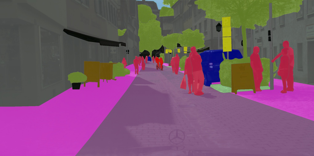
Figure 4-31. In semantic image segmentation, every pixel in the image is assigned a category (like “road,” “sky,” “vegetation,” or “building”). Notice that “people,” for example, is a single class across the whole image. Objects are not individualized. Image from Cityscapes.

For semantic image segmentation, a simple and quite often sufficient approach is called U-Net. The U-Net is a convolutional network architecture that was designed for biomedical image segmentation (see Figure 4-32) and won a cell tracking competition in 2015.

Figure 4-32. The U-Net architecture was designed to segment biomedical images such as these microscopy cell images. Images from Ronneberger et al., 2015.

The U-Net architecture is represented in Figure 4-33. A U-Net consists of an encoder which downsamples an image to an encoding (the lefthand side of architecture), and a mirrored decoder which upsamples the encoding back to the desired mask (the righthand side of the architecture). The decoder blocks have a number of skip connections (depicted by the horizontal arrows in the center) that directly connect from the encoder blocks. These skip connections copy features at a specific resolution and concatenate them channel-wise with specific feature maps in the decoder. This brings information at various levels of semantic granularity from the encoder directly into the decoder. (Note: cropping may be necessary on the skip connections because of slight size misalignments of the feature maps in corresponding levels of the encoder and decoder. Indeed, U-Net uses all convolutions without padding, which means that border pixels are lost at each layer. This design choice is not fundamental though, and padding can be used as well.)

Figure 4-33. The U-Net architecture consists of mirrored encoder and decoder blocks that take on a U shape when depicted as shown here. Skip connections concatenate feature maps along the depth axis (channels). K is the target number of classes.

Images and labels

To illustrate U-Net image segmentation we’ll use the Oxford Pets dataset, where each of the input images contains a label mask as shown in Figure 4-34. The label is an image in which pixels are assigned one of three integer values depending on whether they are background, the object outline, or the object interior.

Figure 4-34. Training images (top row) and labels (bottom row) from the Oxford Pets dataset.

We’ll treat these three pixel values as the index of class labels and train the network to carry out multiclass classification:

model = ...
model.compile(optimizer='adam',
    loss=tf.keras.losses.SparseCategoricalCrossentropy(from_logits=True),
    metrics=['accuracy'])
model.fit(...)

The complete code is available in 04b_unet_segmentation.ipynb on GitHub.

Architecture

Training a U-Net architecture from scratch requires a lot of trainable parameters. As discussed in “Other considerations” it’s difficult to label datasets for tasks such as object detection and segmentation. Therefore, to use the labeled data efficiently, it is better to use a pretrained backbone and employ transfer learning for the encoder block. As in Chapter 3, we can use a pretrained MobileNetV2 to create the encoding:

 base_model = tf.keras.applications.MobileNetV2(
    input_shape=[128, 128, 3], include_top=False)

The decoder side will consist of upsampling layers to get back to the desired mask shape. The decoder also needs feature maps from specific layers of the encoder (skip connections). The layers of the MobileNetV2 model that we need can be obtained by name as follows:

layer_names = [
    'block_1_expand_relu',   # 64x64
    'block_3_expand_relu',   # 32x32
    'block_6_expand_relu',   # 16x16
    'block_13_expand_relu',  # 8x8
    'block_16_project',      # 4x4
]
base_model_outputs = [base_model.get_layer(name).output for name in layer_names]

The “down stack” or lefthand side of the U-Net architecture then consists of the image as input, and these layers as outputs. We are carrying out transfer learning, so the entire lefthand side does not need weight adjustments:

down_stack = tf.keras.Model(inputs=base_model.input,
                            outputs=base_model_outputs,
                            name='pretrained_mobilenet')
down_stack.trainable = False

Upsampling in Keras can be accomplished using a Conv2DTranspose layer. We also add batch normalization and nonlinearity to each step of the upsampling:

def upsample(filters, size, name):
  return tf.keras.Sequential([
     tf.keras.layers.Conv2DTranspose(filters, size,
                                     strides=2, padding='same'),
     tf.keras.layers.BatchNormalization(),
     tf.keras.layers.ReLU()
  ], name=name)

up_stack = [
    upsample(512, 3, 'upsample_4x4_to_8x8'),
    upsample(256, 3, 'upsample_8x8_to_16x16'),
    upsample(128, 3, 'upsample_16x16_to_32x32'),
    upsample(64, 3,  'upsample_32x32_to_64x64')
]

Each stage of the decoder up stack is concatenated with the corresponding layer of the encoder down stack:

for up, skip in zip(up_stack, skips):
    x = up(x)
    concat = tf.keras.layers.Concatenate()
    x = concat([x, skip])

Training

We can display the predictions on a few selected images using a Keras callback:

class DisplayCallback(tf.keras.callbacks.Callback):
  def on_epoch_end(self, epoch, logs=None):
      show_predictions(train_dataset, 1)

model.fit(train_dataset, ...,
          callbacks=[DisplayCallback()])

The result of doing so on the Oxford Pets dataset is shown in Figure 4-35. Note that the model starts out with garbage (top row), as one would expect, but then learns which pixels correspond to the animal and which pixels correspond to the background.

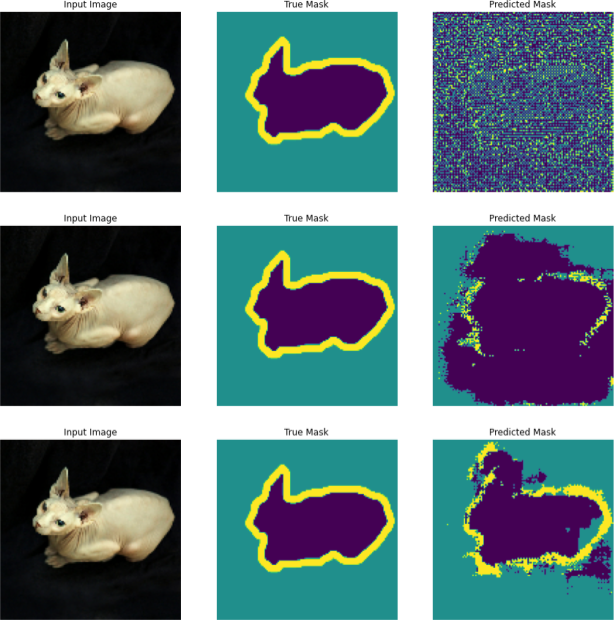
Figure 4-35. The predicted mask on the input image improves epoch by epoch as the model is trained.

However, because the model is trained to predict each pixel as background, outline, or interior independently of the other pixels, we see artifacts such as unclosed regions and disconnected pixels. The model doesn’t realize that the region corresponding to the cat should be closed. That is why this approach is mostly used on images where the segments to be detected do not need to be contiguous, like the example in Figure 4-31, where the “road,” “sky,” and “vegetation” segments often have discontinuities.

An example of an application is in self-driving algorithms, to detect the road. Another is in satellite imagery, where a U-Net architecture was used to solve the hard problem of distinguishing clouds from snow; both are white, but snow coverage is useful ground-level information, whereas cloud obstruction means that the image needs to be retaken.

Current Research Directions

For object detection, a recent landmark is EfficientDet, which builds an object detection architecture on top of the EfficientNet backbone. Apart from the backbone, it brings a new class of multilayer FPNs called the bi-directional feature pyramid network (BiFPN).

For semantic segmentation, U-Net is the simplest but not the state-of-the-art architecture. You can read about more complex approaches in the papers on DeepLabv3 and the pyramid scene parsing network (PSPNet). DeepLabv3 is currently considered state of the art for image segmentation and is the architecture implemented in the TensorFlow Model Garden.

Kirillov et al. recently opened up a new field in object detection with their proposed panoptic segmentation task, which combines instance segmentation and full-scene semantic segmentation into a single model. Objects are classified in two ways: either countable objects like “persons” or “cars” that are detected individually, or uncountable types of objects like “the road” or “the sky” which are segmented globally. The current top approaches in this domain are Panoptic FPN and Panoptic DeepLab, both implemented as part of the Detectron2 platform.

Summary

In this chapter, we looked at object detection and image segmentation methods. We started with YOLO, considering its limitations, and then discussed RetinaNet, which innovates over YOLO in terms of both the architecture and the losses used. We also discussed Mask R-CNN to carry out instance segmentation and U-Net to carry out semantic segmentation.

In the next chapters, we will delve more deeply into different parts of the computer vision pipeline using the simple transfer learning image classification architecture from Chapter 3 as our core model. The pipeline steps remain the same regardless of the backbone architecture or the problem being solved.