To be able to improve the performance of your system you need a prior understanding of what can be improved, how it can be improved, how much it can be improved, and, most importantly, what impact the improvement will have on the overall performance of your system. You need to be able to identify those things that, after you have done your best to improve them, will yield substantial benefits for the overall system performance. Concentrate your efforts on them, and avoid wasting time on improvements that give little overall gain.
If you have a small application it may be possible to detect places that could be improved simply by inspecting the code. On the other hand, if you have a large application, or many applications, it’s usually impossible to do the detective work with the naked eye. You need observation instruments and measurement tools. These belong to the benchmarking and code-profiling categories.
It’s important to understand that in the majority of the benchmarking tests that we will execute, we will not be looking at absolute results. Few machines will have exactly the same hardware and software setup, so this kind of comparison would usually be misleading, and in most cases we will be trying to show which coding approach is preferable, so the hardware is almost irrelevant.
Rather than looking at absolute results, we will be looking at the differences between two or more result sets run on the same machine. This is what you should do; you shouldn’t try to compare the absolute results collected here with the results of those same benchmarks on your own machines.
In this chapter we will present a few existing tools that are widely used; we will apply them to example code snippets to show you how performance can be measured, monitored, and improved; and we will give you an idea of how you can develop your own tools.
As web service developers, the most important thing we should strive for is to offer the user a fast, trouble-free browsing experience. Measuring the response rates of our servers under a variety of load conditions and benchmark programs helps us to do this.
A benchmark program may consume significant resources, so you cannot find the real times that a typical user will wait for a response from your service by running the benchmark on the server itself. Ideally you should run it from a different machine. A benchmark program is unlike a typical user in the way it generates requests. It should be able to emulate multiple concurrent users connecting to the server by generating many concurrent requests. We want to be able to tell the benchmark program what load we want to emulate—for example, by specifying the number or rate of requests to be made, the number of concurrent users to emulate, lists of URLs to request, and other relevant arguments.
ApacheBench (ab) is a tool for benchmarking your Apache HTTP server. It is designed to give you an idea of the performance that your current Apache installation can give. In particular, it shows you how many requests per second your Apache server is capable of serving. The ab tool comes bundled with the Apache source distribution, and like the Apache web server itself, it’s free.
Let’s try it. First we create a test script, as shown in Example 9-1.
We will simulate 10 users concurrently requesting the file simple_test.pl through http://localhost/perl/simple_test.pl. Each simulated user makes 500 requests. We generate 5,000 requests in total:
panic% ./ab -n 5000 -c 10 http://localhost/perl/simple_test.pl

Server Software:        Apache/1.3.25-dev
Server Hostname:        localhost
Server Port:            8000

Document Path:          /perl/simple_test.pl
Document Length:        6 bytes

Concurrency Level:      10
Time taken for tests:   5.843 seconds
Complete requests:      5000
Failed requests:        0
Broken pipe errors:     0
Total transferred:      810162 bytes
HTML transferred:       30006 bytes
Requests per second:    855.72 [#/sec] (mean)
Time per request:       11.69 [ms] (mean)
Time per request:       1.17 [ms] (mean, across all concurrent requests)
Transfer rate:          138.66 [Kbytes/sec] received

Connnection Times (ms)
              min  mean[+/-sd] median   max
Connect:        0     1    1.4      0    17
Processing:     1    10   12.9      7   208
Waiting:        0     9   13.0      7   208
Total:          1    11   13.1      8   208
Most of the report is not very interesting to us. What we really care about are the Requests per second and Connection Times results:
- Requests per second
The number of requests (to our test script) the server was able to serve in one second
- Connect and Waiting times
The amount of time it took to establish the connection and get the first bits of a response
- Processing time
The server response time—i.e., the time it took for the server to process the request and send a reply
- Total time
The sum of the Connect and Processing times
As you can see, the server was able to respond on average to 856 requests per second. On average, it took no time to establish a connection to the server both the client and the server are running on the same machine and 10 milliseconds to process each request. As the code becomes more complicated you will see that the processing time grows while the connection time remains constant. The latter isn’t influenced by the code complexity, so when you are working on your code performance, you care only about the processing time. When you are benchmarking the overall service, you are interested in both.
Just for fun, let’s benchmark a similar script, shown in Example 9-2, under mod_cgi.
Example 9-2. simple_test_mod_cgi.pl
#!/usr/bin/perl
print "Content-type: text/plain\n\n";
print "Hello\n";
The script is configured as:
ScriptAlias /cgi-bin/ /usr/local/apache/cgi-bin/

panic% /usr/local/apache/bin/ab -n 5000 -c 10 \
http://localhost/cgi-bin/simple_test_mod_cgi.pl
We will show only the results that interest us:
Requests per second:    156.40 [#/sec] (mean)
Time per request:       63.94 [ms] (mean)
Now, when essentially the same script is executed under mod_cgi instead of mod_perl, we get 156 requests per second responded to, not 856.
ApacheBench can generate KeepAlives,
GET (default) and POST
requests, use Basic Authentication, send cookies
and custom HTTP headers. The version of
ApacheBench released with Apache version 1.3.20
adds SSL support, generates gnuplot and CSV
output for postprocessing, and reports median and standard deviation
values.
HTTPD::Bench::ApacheBench, available
from CPAN, provides a Perl interface
for ab.
httperf is another tool for measuring web server performance. Its input and reports are different from the ones we saw while using ApacheBench. This tool’s manpage includes an in-depth explanation of all the options it accepts and the results it generates. Here we will concentrate on the input and on the part of the output that is most interesting to us.
With httperf you cannot specify the concurrency level; instead, you have to specify the connection opening rate (—rate) and the number of calls (—num-call) to perform on each opened connection. To compare the results we received from ApacheBench we will use a connection rate slightly higher than the number of requests responded to per second reported by ApacheBench. That number was 856, so we will try a rate of 860 (—rate 860) with just one request per connection (—num-call 1). As in the previous test, we are going to make 5,000 requests (—num-conn 5000). We have set a timeout of 60 seconds and allowed httperf to use as many ports as it needs (—hog).
So let’s execute the benchmark and analyze the results:
panic% httperf --server localhost --port 80 --uri /perl/simple_test.pl \
--hog --rate 860 --num-conn 5000 --num-call 1 --timeout 60

Maximum connect burst length: 11

Total: connections 5000 requests 5000 replies 5000 test-duration 5.854 s

Connection rate: 854.1 conn/s (1.2 ms/conn, <=50 concurrent connections)
Connection time [ms]: min 0.8 avg 23.5 max 226.9 median 20.5 stddev 13.7
Connection time [ms]: connect 4.0
Connection length [replies/conn]: 1.000

Request rate: 854.1 req/s (1.2 ms/req)
Request size [B]: 79.0

Reply rate [replies/s]: min 855.6 avg 855.6 max 855.6 stddev 0.0 (1 samples)
Reply time [ms]: response 19.5 transfer 0.0
Reply size [B]: header 184.0 content 6.0 footer 2.0 (total 192.0)
Reply status: 1xx=0 2xx=5000 3xx=0 4xx=0 5xx=0

CPU time [s]: user 0.33 system 1.53 (user 5.6% system 26.1% total 31.8%)
Net I/O: 224.4 KB/s (1.8*10^6 bps)

Errors: total 0 client-timo 0 socket-timo 0 connrefused 0 connreset 0
Errors: fd-unavail 0 addrunavail 0 ftab-full 0 other 0
As before, we are mostly interested in the average Reply rate—855, almost exactly the same result reported by ab in the previous section. Notice that when we tried —rate 900 for this particular setup, the reported request rate went down drastically, since the server’s performance gets worse when there are more requests than it can handle.
http_load is yet another utility that does web server load testing. It can simulate a 33.6 Kbps modem connection (-throttle) and allows you to provide a file with a list of URLs that will be fetched randomly. You can specify how many parallel connections to run (-parallel N) and the number of requests to generate per second (-rate N). Finally, you can tell the utility when to stop by specifying either the test time length (-seconds N) or the total number of fetches (-fetches N).
Again, we will try to verify the results reported by ab (claiming that the script under test can handle about 855 requests per second on our machine). Therefore we run http_load with a rate of 860 requests per second, for 5 seconds in total. We invoke is on the file urls, containing a single URL:
http://localhost/perl/simple_test.pl
Here is the generated output:
panic% http_load -rate 860 -seconds 5 urls
4278 fetches, 325 max parallel, 25668 bytes, in 5.00351 seconds
6 mean bytes/connection
855 fetches/sec, 5130 bytes/sec
msecs/connect: 20.0881 mean, 3006.54 max, 0.099 min
msecs/first-response: 51.3568 mean, 342.488 max, 1.423 min
HTTP response codes:
  code 200 -- 4278
This application also reports almost exactly the same response-rate capability: 855 requests per second. Of course, you may think that it’s because we have specified a rate close to this number. But no, if we try the same test with a higher rate:
panic% http_load -rate 870 -seconds 5 urls
4045 fetches, 254 max parallel, 24270 bytes, in 5.00735 seconds
6 mean bytes/connection
807.813 fetches/sec, 4846.88 bytes/sec
msecs/connect: 78.4026 mean, 3005.08 max, 0.102 min
we can see that the performance goes down—it reports a response rate of only 808 requests per second.
The nice thing about this utility is that you can list a few URLs to test. The URLs that get fetched are chosen randomly from the specified file.
Note that when you provide a file with a list of URLs, you must make sure that you don’t have empty lines in it. If you do, the utility will fail and complain:
./http_load: unknown protocol -
The following are also interesting benchmarking applications implemented in Perl:
-
HTTP::WebTest The
HTTP::WebTestmodule (available from CPAN) runs tests on remote URLs or local web files containing Perl, JSP, HTML, JavaScript, etc. and generates a detailed test report.-
HTTP::Monkeywrench HTTP::Monkeywrenchis a test-harness application to test the integrity of a user’s path through a web site.-
Apache::RecorderandHTTP::RecordedSession Apache::Recorder(available from CPAN) is a mod_perl handler that records an HTTP session and stores it on the web server’s filesystem.HTTP::RecordedSessionreads the recorded session from the filesystem and formats it for playback usingHTTP::WebTestorHTTP::Monkeywrench. This is useful when writing acceptance and regression tests.
Many other benchmark utilities are available both for free and for
money. If you find that none of these suits your needs,
it’s quite easy to roll your own utility. The
easiest way to do this is to write a Perl script that uses the
LWP::Parallel::UserAgent and
Time::HiRes modules. The former module allows you
to open many parallel connections and the latter allows you to take
time samples with microsecond resolution.
If you want
to benchmark your Perl code, you can use
the Benchmark module. For example,
let’s say that our code generates many long strings
and finally prints them out. We wonder what is the most efficient way
to handle this task—we can try to concatenate the strings into
a single string, or we can store them (or references to them) in an
array before generating the output. The easiest way to get an answer
is to try each approach, so we wrote the benchmark shown in Example 9-3.
Example 9-3. strings_benchmark.pl
use Benchmark;
use Symbol;
my $fh = gensym;

open $fh, ">/dev/null" or die $!;

my($one, $two, $three) = map { $_ x 4096 } 'a'..'c';

timethese(100_000, {
    ref_array => sub {
        my @a;
        push @a, \($one, $two, $three);
        my_print(@a);
    },
    array => sub {
        my @a;
        push @a, $one, $two, $three;
        my_print(@a);
    },
    concat => sub {
        my $s;
        $s .= $one;
        $s .= $two;
        $s .= $three;
        my_print($s);
    },
});
sub my_print {
    for (@_) {
        print $fh ref($_) ? $$_ : $_;
    }
}
As you can see, we generate three big strings and then use three
anonymous functions to print them out. The first one
(ref_array) stores the references to the strings
in an array. The second function (array) stores
the strings themselves in an array. The third function
(concat) concatenates the three strings into a
single string. At the end of each function we print the stored data.
If the data structure includes references, they are first
dereferenced (relevant for the first function only). We execute each
subtest 100,000 times to get more precise results. If your results
are too close and are below 1 CPU clocks, you should try setting the
number of iterations to a bigger number. Let’s
execute this benchmark and check the results:
panic% perl strings_benchmark.pl
Benchmark: timing 100000 iterations of array, concat, ref_array...
     array:  2 wallclock secs ( 2.64 usr +  0.23 sys =  2.87 CPU)
    concat:  2 wallclock secs ( 1.95 usr +  0.07 sys =  2.02 CPU)
 ref_array:  3 wallclock secs ( 2.02 usr +  0.22 sys =  2.24 CPU)
First, it’s important to remember that the reported wallclock times can be misleading and thus should not be relied upon. If during one of the subtests your computer was more heavily loaded than during the others, it’s possible that this particular subtest will take more wallclocks to complete, but this doesn’t matter for our purposes. What matters is the CPU clocks, which tell us the exact amount of CPU time each test took to complete. You can also see the fraction of the CPU allocated to usr and sys, which stand for the user and kernel (system) modes, respectively. This tells us what proportions of the time the subtest has spent running code in user mode and in kernel mode.
Now that you know how to read the results, you can see that concatenation outperforms the two array functions, because concatenation only has to grow the size of the string, whereas array functions have to extend the array and, during the print, iterate over it. Moreover, the array method also creates a string copy before appending the new element to the array, which makes it the slowest method of the three.
Let’s make the strings much smaller. Using our original code with a small correction:
my($one, $two, $three) = map { $_ x 8 } 'a'..'c';we now make three strings of 8 characters, instead of 4,096. When we execute the modified version we get the following picture:
Benchmark: timing 100000 iterations of array, concat, ref_array...
     array:  1 wallclock secs ( 1.59 usr +  0.01 sys =  1.60 CPU)
    concat:  1 wallclock secs ( 1.16 usr +  0.04 sys =  1.20 CPU)
 ref_array:  2 wallclock secs ( 1.66 usr +  0.05 sys =  1.71 CPU)
Concatenation still wins, but this time the array method is a bit
faster than ref_array, because the overhead of taking string
references before pushing them into an array and dereferencing them
afterward during print( ) is bigger than the
overhead of making copies of the short strings.
As these examples show, you should benchmark your code by rewriting parts of the code and comparing the benchmarks of the modified and original versions.
Also note that benchmarks can give different results under different versions of the Perl interpreter, because each version might have built-in optimizations for some of the functions. Therefore, if you upgrade your Perl interpreter, it’s best to benchmark your code again. You may see a completely different result.
Another Perl code benchmarking method is to use the
Time::HiRes
module, which allows you to get the
runtime of your code with a fine-grained resolution of the order of
microseconds. Let’s compare a few methods to
multiply two numbers (see Example 9-4).
Example 9-4. hires_benchmark_time.pl
use Time::HiRes qw(gettimeofday tv_interval);
my %subs = (
    obvious => sub {
        $_[0] * $_[1]
    },
    decrement => sub {
        my $a = shift;
        my $c = 0;
        $c += $_[0] while $a--;
        $c;
    },
);

for my $x (qw(10 100)) {
    for my $y (qw(10 100)) {
        for (sort keys %subs) {
            my $start_time = [ gettimeofday ];
            my $z = $subs{$_}->($x,$y);
            my $end_time = [ gettimeofday ];
            my $elapsed = tv_interval($start_time,$end_time);
            printf "%-9.9s: Doing %3.d * %3.d = %5.d took %f seconds\n",
                $_, $x, $y, $z, $elapsed;
        }
        print "\n";
    }
}
We have used two methods here. The first (obvious)
is doing the normal multiplication, $z=$x*$y. The
second method is using a trick of the systems where there is no
built-in multiplication function available; it uses only the addition
and subtraction operations. The trick is to add $x
for $y times (as you did in school before you
learned multiplication).
When we execute the code, we get:
panic% perl hires_benchmark_time.pl
decrement: Doing  10 *  10 =   100 took 0.000064 seconds
obvious  : Doing  10 *  10 =   100 took 0.000016 seconds

decrement: Doing  10 * 100 =  1000 took 0.000029 seconds
obvious  : Doing  10 * 100 =  1000 took 0.000013 seconds

decrement: Doing 100 *  10 =  1000 took 0.000098 seconds
obvious  : Doing 100 *  10 =  1000 took 0.000013 seconds

decrement: Doing 100 * 100 = 10000 took 0.000093 seconds
obvious  : Doing 100 * 100 = 10000 took 0.000012 seconds
Note that if the processor is very fast or the OS has a coarse time-resolution granularity (i.e., cannot count microseconds) you may get zeros as reported times. This of course shouldn’t be the case with applications that do a lot more work.
If you run this benchmark again, you will notice that the numbers
will be slightly different. This is because the code measures
absolute time, not the real execution time (unlike the previous
benchmark using the Benchmark module).
You can see that doing 10*100 as opposed to
100*10 results in quite different results for the
decrement method. When the arguments are 10*100,
the code performs the add 100 operation only 10
times, which is obviously faster than the second invocation,
100*10, where the code performs the add
10 operation 100 times. However, the normal multiplication
takes a constant time.
Let’s run the same code using the
Benchmark module, as shown in Example 9-5.
Example 9-5. hires_benchmark.pl
use Benchmark;
my %subs = (
    obvious => sub {
        $_[0] * $_[1]
    },
    decrement => sub {
        my $a = shift;
        my $c = 0;
        $c += $_[0] while $a--;
        $c;
    },
);

for my $x (qw(10 100)) {
    for my $y (qw(10 100)) {
        print "\nTesting $x*$y\n";
        timethese(300_000, {
            obvious   => sub {$subs{obvious}->($x, $y)  },
            decrement => sub {$subs{decrement}->($x, $y)},
        });
    }
}
Now let’s execute the code:
panic% perl hires_benchmark.pl
Testing 10*10
Benchmark: timing 300000 iterations of decrement, obvious...
 decrement:  4 wallclock secs ( 4.27 usr +  0.09 sys =  4.36 CPU)
   obvious:  1 wallclock secs ( 0.91 usr +  0.00 sys =  0.91 CPU)

Testing 10*100
Benchmark: timing 300000 iterations of decrement, obvious...
 decrement:  5 wallclock secs ( 3.74 usr +  0.00 sys =  3.74 CPU)
   obvious:  0 wallclock secs ( 0.87 usr +  0.00 sys =  0.87 CPU)

Testing 100*10
Benchmark: timing 300000 iterations of decrement, obvious...
 decrement: 24 wallclock secs (24.41 usr +  0.00 sys = 24.41 CPU)
   obvious:  2 wallclock secs ( 0.86 usr +  0.00 sys =  0.86 CPU)

Testing 100*100
Benchmark: timing 300000 iterations of decrement, obvious...
 decrement: 23 wallclock secs (23.64 usr +  0.07 sys = 23.71 CPU)
   obvious:  0 wallclock secs ( 0.80 usr +  0.00 sys =  0.80 CPU)
You can observe exactly the same behavior, but this time using the
average CPU clocks collected over 300,000 tests and not the absolute
time collected over a single sample. Obviously, you can use the
Time::HiRes module in a benchmark that will
execute the same code many times to report a more precise runtime,
similar to the way the Benchmark module reports
the CPU time.
However, there are situations where getting the average speed is not
enough. For example, if you’re testing some code
with various inputs and calculate only the average processing times,
you may not notice that for some particular inputs the code is very
ineffective. Let’s say that the average is 0.72
seconds. This doesn’t reveal the possible fact that
there were a few cases when it took 20 seconds to process the input.
Therefore, getting the variance[1] in addition to the average may be important.
Unfortunately Benchmark.pm cannot provide such
results—system timers are rarely good enough to measure fast
code that well, even on single-user systems, so you must run the code
thousands of times to get any significant CPU time. If the code is
slow enough that each single execution can be measured, most likely
you can use the profiling
tools.
A very important aspect of performance tuning is to make sure that your applications don’t use too much memory. If they do, you cannot run many servers, and therefore in most cases, under a heavy load the overall performance will be degraded. The code also may leak memory, which is even worse, since if the same process serves many requests and more memory is used after each request, after a while all the RAM will be used and the machine will start swapping (i.e., using the swap partition). This is a very undesirable situation, because when the system starts to swap, the performance will suffer badly. If memory consumption grows without bound, it will eventually lead to a machine crash.
The simplest way to figure out how big the processes are and to see whether they are growing is to watch the output of the top(1) or ps(1) utilities.
For example, here is the output of top(1):
8:51am  up 66 days,  1:44,  1 user,  load average: 1.09, 2.27, 2.61
  95 processes: 92 sleeping, 3 running, 0 zombie, 0 stopped
  CPU states: 54.0% user,  9.4% system,  1.7% nice, 34.7% idle
  Mem:  387664K av, 309692K used,  77972K free, 111092K shrd,  70944K buff
  Swap: 128484K av,  11176K used, 117308K free                170824K cached

 PID USER PRI NI SIZE  RSS SHARE STAT LIB %CPU %MEM   TIME COMMAND
  29225 nobody 0  0  9760 9760  7132 S      0 12.5  2.5   0:00 httpd_perl
  29220 nobody 0  0  9540 9540  7136 S      0  9.0  2.4   0:00 httpd_perl
  29215 nobody 1  0  9672 9672  6884 S      0  4.6  2.4   0:01 httpd_perl
  29255 root   7  0  1036 1036   824 R      0  3.2  0.2   0:01 top
376 squid  0  0 15920  14M   556 S      0  1.1  3.8 209:12 squid
  29227 mysql  5  5  1892 1892   956 S N    0  1.1  0.4   0:00 mysqld
  29223 mysql  5  5  1892 1892   956 S N    0  0.9  0.4   0:00 mysqld
  29234 mysql  5  5  1892 1892   956 S N    0  0.9  0.4   0:00 mysqld
This starts with overall information about the system and then
displays the most active processes at the given moment. So, for
example, if we look at the httpd_perl processes,
we can see the size of the resident (RSS) and
shared (SHARE) memory segments.[2] This sample was
taken on a production server running Linux.
But of course we want to see all the apache/mod_perl processes, and that’s where ps(1) comes in. The options of this utility vary from one Unix flavor to another, and some flavors provide their own tools. Let’s check the information about mod_perl processes:
panic% ps -o pid,user,rss,vsize,%cpu,%mem,ucomm -C httpd_perl
  PID USER      RSS   VSZ %CPU %MEM COMMAND
29213 root     8584 10264  0.0  2.2 httpd_perl
29215 nobody   9740 11316  1.0  2.5 httpd_perl
29216 nobody   9668 11252  0.7  2.4 httpd_perl
29217 nobody   9824 11408  0.6  2.5 httpd_perl
29218 nobody   9712 11292  0.6  2.5 httpd_perl
29219 nobody   8860 10528  0.0  2.2 httpd_perl
29220 nobody   9616 11200  0.5  2.4 httpd_perl
29221 nobody   8860 10528  0.0  2.2 httpd_perl
29222 nobody   8860 10528  0.0  2.2 httpd_perl
29224 nobody   8860 10528  0.0  2.2 httpd_perl
29225 nobody   9760 11340  0.7  2.5 httpd_perl
29235 nobody   9524 11104  0.4  2.4 httpd_perl
Now you can see the resident (RSS) and virtual
(VSZ) memory segments (and the shared memory
segment if you ask for it) of all mod_perl processes. Please refer to
the top(1) and ps(1)
manpages for more information.
You probably agree that using top(1) and
ps(1) is cumbersome if you want to use
memory-size sampling during the benchmark test. We want to have a way
to print memory sizes during program execution at the desired places.
The GTop module, which is a Perl glue to the
libgtop library, is exactly what we need for that
task.
You are fortunate if you run Linux or any of the BSD flavors, as the
libgtop
C library from the GNOME project is
supported on those platforms. This library provides an API to access
various system-wide and process-specific information. (Some other
operating systems also support libgtop.)
With GTop
, if we want to print the memory size of
the current process we’d just execute:
use GTop ( );
print GTop->new->proc_mem($$)->size;
$$
is the Perl special variable that gives
the process ID (PID) of the currently running process.
If you want to look at some other process and you have the necessary
permission, just replace $$ with the other
process’s PID and you can peek inside it. For
example, to check the shared size, you’d do:
print GTop->new->proc_mem($$)->share;
Let’s try to run some tests:
panic% perl -MGTop -e 'my $g = GTop->new->proc_mem($$); \
  printf "%5.5s => %d\n",$_,$g->$_( ) for qw(size share vsize rss)'

 size => 1519616
share => 1073152
vsize => 2637824
  rss => 1515520
We have just printed the memory sizes of the process: the real, the shared, the virtual, and the resident (not swapped out).
There are many other things GTop can do for
you—please refer to its manpage for more information. We are
going to use this module in our performance tuning tips later in this
chapter, so you will be able to exercise it a lot.
If you are running a true BSD system, you may use
BSD::Resource::getrusage
instead of GTop. For example:
print "used memory = ".(BSD::Resource::getrusage)[2]."\n"
For more information, refer to the BSD::Resource
manpage.
The
Apache::VMonitor
module, with the help of the
GTop module, allows you to watch all your system
information using your favorite browser, from anywhere in the world,
without the need to telnet to your machine. If
you are wondering what information you can retrieve with
GTop, you should look at
Apache::VMonitor, as it utilizes a large part of
the API GTop
provides.
The Apache::Status
module allows
you to peek inside the Perl interpreter in the Apache web server. You
can watch the status of the Perl interpreter: what modules and
Registry scripts are compiled in, the content of variables, the sizes
of the subroutines, and more.
To configure this module you should add the following section to your httpd.conf file:
<Location /perl-status>
    SetHandler perl-script
    PerlHandler +Apache::Status
</Location>
and restart Apache.
Now when you access the location http://localhost:8000/perl-status you will see a menu (shown in Figure 9-1) that leads you into various sections that will allow you to explore the innards of the Perl interpreter.
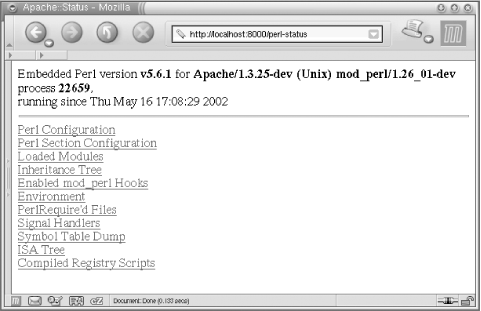
When you use this module for debugging, it’s best to run the web server in single-server mode (httpd -X). If you don’t you can get confused, because various child processes might show different information. It’s simpler to work with a single process.
To enable the Apache::Status modules to present
more exotic information, make sure that the following modules are
installed: Data::Dumper,
Apache::Peek, Devel::Peek,
B::LexInfo, B::Deparse,
B::Terse, and B::TerseSize.
Some of these modules are bundled with Perl; others should be
installed by hand.
When you have the aforementioned modules installed, add these directives to your httpd.conf file:
PerlSetVar StatusOptionsAll On
PerlSetVar StatusDumper On
PerlSetVar StatusPeek On
PerlSetVar StatusLexInfo On
PerlSetVar StatusDeparse On
PerlSetVar StatusDeparseOptions "-p -sC"
PerlSetVar StatusTerse On
PerlSetVar StatusTerseSize On
PerlSetVar StatusTerseSizeMainSummary On
and restart Apache. Alternatively, if you enable all the options, you
can use the option StatusOptionsAll to replace all
the options that can be On or
Off, so you end up with just these two lines:
PerlSetVar StatusOptionsAll On
PerlSetVar StatusDeparseOptions "-p -sC"
When you explore the contents of the compiled Perl module or Registry script, at the bottom of the screen you will see a Memory Usage link. When you click on it, you will be presented with a list of funtions in the package. For each function, the size and the number of OP codes will be shown.
For example, let’s create a module that prints the
contents of the %ENV hash. This module is shown in
Example 9-6.
Example 9-6. Book/DumpEnv.pm
package Book::DumpEnv;
use strict;
use Apache::Constants qw(:common);
sub handler {
    shift->send_http_header('text/plain');
    print map {"$_ => $ENV{$_}\n"} keys %ENV;
    return OK;
}
1;
Now add the following to httpd.conf:
<Location /dumpenv>
    SetHandler perl-script
    PerlHandler +Book::DumpEnv
</Location>
Restart the server in single-server mode (httpd
-X), request the URL
http://localhost:8000/dumpenv, and you will see
that the contents of %ENV are displayed.
Now it’s time to peek inside the
Book::DumpEnv package inside the Perl interpreter.
Issue the request to
http://localhost:8000/perl-status, click on the
“Loaded Modules” menu item, and
locate Book::DumpEnv on the displayed page. Click
on it to request a page at the URI
http://localhost:8000/perl-status?Book::DumpEnv.
You will see the screen shown in Figure 9-2.
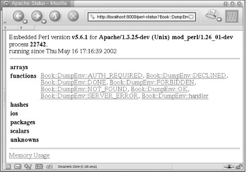
You can see seven functions that were imported with:
use Apache::Constants qw(:common);
and a single function that we have created, called
handler. No other Perl variable types were created
in the package Book::DumpEnv.
Now click on the “Memory Usage” link at the bottom of the page. The screen shown in Figure 9-3 will be rendered.
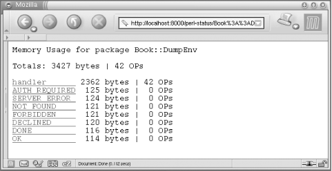
So you can see that Book::DumpEnv takes 3,427
bytes in memory, whereas the handler function
takes 2,362 bytes.
Is this all? No, we can go even further inside the code and learn the
syntax tree size (i.e., what opcodes construct each line of the
source code and how many bytes each source-code line consumes). If we
click on handler we will see the syntax tree of
this function, and how much memory each Perl OPcode and line of code
take. For example, in Figure 9-4 we can see that
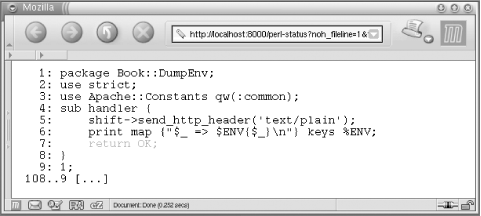
line 7, which corresponds to this source-code line in
Book/DumpEnv.pm:
7: return OK;
takes up 136 bytes of memory.
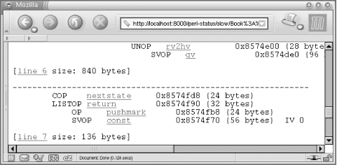
We found the corresponding source-code line by clicking the “line 7” hyperlink shown in Figure 9-4, which displays the source code of the module with the relevant line highlighted (see Figure 9-5).
Now you should be able to to find out how much memory each subroutine or even each individual source line of Perl code consumes. This will allow you to optimize memory usage by comparing several implemenations of the same algorithm and choosing the one that consumes the smallest amount of memory.
The profiling process helps you to determine which subroutines (or just snippets of code) take longest to execute and which subroutines are called most often. You will probably want to optimize these.
When do you need to profile your code? You do that when you suspect that some part of your code is called very often and maybe there is a need to optimize it, which could significantly improve the overall performance.
Devel::DProf
collects
information on the execution time of a Perl script and of the
subroutines in that script.
Let’s take for example the
diagnostics pragma and measure the impact of its
usage on the program compilation and execution speed. This pragma
extends the terse diagnostics normally emitted by both the Perl
compiler and the Perl interpreter, augmenting them with the more
verbose and endearing descriptions found in the
perldiag manpage. We have claimed that this
pragma should not be used on a production server. We are going to use
Devel::DProf to explain our claim.
We will run a benchmark, once with diagnostics enabled and once
disabled, on a subroutine called test_code( ).
The code inside the subroutine does either a lexical or a numeric
comparison of two strings. It assigns one string to another if the
condition tests true, but the condition is always false. To
demonstrate the diagnostics pragma overhead, the
comparison operator that we use in Example 9-7 is
intentionally wrong. It should be a string comparison
(eq), and we use a numeric one (=
=).
Example 9-7. bench_diagnostics.pl
use Benchmark;
use diagnostics;
use strict;

my $count = 50000;

disable diagnostics;
my $t1 = timeit($count,\&test_code);

enable  diagnostics;
my $t2 = timeit($count,\&test_code);

print "Off: ",timestr($t1),"\n";
print "On : ",timestr($t2),"\n";

sub test_code {
    my ($a, $b) = qw(foo bar);
    my $c;
    if ($a =  = $b) {
        $c = $a;
    }
}
For only a few lines of code we get:
Off:  1 wallclock secs ( 0.81 usr +  0.00 sys =  0.81 CPU)
On : 13 wallclock secs (12.54 usr +  0.01 sys = 12.55 CPU)
With diagnostics enabled, the subroutine test_code(
) is 16 times slower (12.55/0.81: remember that
we’re talking in CPU time, not wallclock seconds)
than with diagnostics disabled!
Now let’s fix the comparison the way it should be,
by replacing = = with eq, so we
get:
my ($a, $b) = qw(foo bar);
my $c;
if ($a eq $b) {
$c = $a;
}and run the same benchmark again:
Off: 1 wallclock secs ( 0.57 usr + 0.00 sys = 0.57 CPU) On : 1 wallclock secs ( 0.56 usr + 0.00 sys = 0.56 CPU)
Now there is no overhead at all. The diagnostics
pragma slows things down only when warnings are generated.
After we have verified that using the diagnostics
pragma might add a big overhead to execution runtime,
let’s use code profiling to understand why this
happens. We use Devel::DProf to profile the code
shown in Example 9-8.
Example 9-8. diagnostics.pl
use diagnostics;
test_code( );
sub test_code {
my($a, $b) = qw(foo bar);
my $c;
if ($a = = $b) {
$c = $a;
}
}Run it with the profiler enabled, and then create the profiling statistics with the help of dprofpp:
panic% perl -d:DProf diagnostics.pl
panic% dprofpp

Total Elapsed Time = 0.342236 Seconds
  User+System Time = 0.335420 Seconds
Exclusive Times
%Time ExclSec CumulS #Calls sec/call Csec/c  Name
 92.1   0.309  0.358      1   0.3089 0.3578  main::BEGIN
 14.9   0.050  0.039   3161   0.0000 0.0000  diagnostics::unescape
 2.98   0.010  0.010      2   0.0050 0.0050  diagnostics::BEGIN
 0.00   0.000 -0.000      2   0.0000      -  Exporter::import
 0.00   0.000 -0.000      2   0.0000      -  Exporter::export
 0.00   0.000 -0.000      1   0.0000      -  Config::BEGIN
 0.00   0.000 -0.000      1   0.0000      -  Config::TIEHASH
 0.00   0.000 -0.000      2   0.0000      -  Config::FETCH
 0.00   0.000 -0.000      1   0.0000      -  diagnostics::import
 0.00   0.000 -0.000      1   0.0000      -  main::test_code
 0.00   0.000 -0.000      2   0.0000      -  diagnostics::warn_trap
 0.00   0.000 -0.000      2   0.0000      -  diagnostics::splainthis
 0.00   0.000 -0.000      2   0.0000      -  diagnostics::transmo
 0.00   0.000 -0.000      2   0.0000      -  diagnostics::shorten
 0.00   0.000 -0.000      2   0.0000      -  diagnostics::autodescribe
It’s not easy to see what is responsible for this
enormous overhead, even if main::BEGIN seems to be
running most of the time. To get the full picture we must see the OPs
tree, which shows us who calls whom, so we run:
panic% dprofpp -T
The output is:
main::BEGIN
  diagnostics::BEGIN
     Exporter::import
        Exporter::export
  diagnostics::BEGIN
     Config::BEGIN
     Config::TIEHASH
     Exporter::import
        Exporter::export
  Config::FETCH
  Config::FETCH
  diagnostics::unescape
  .....................
  3159 times [diagnostics::unescape] snipped
  .....................
  diagnostics::unescape
  diagnostics::import
diagnostics::warn_trap
  diagnostics::splainthis
     diagnostics::transmo
     diagnostics::shorten
     diagnostics::autodescribe
main::test_code
  diagnostics::warn_trap
     diagnostics::splainthis
        diagnostics::transmo
        diagnostics::shorten
        diagnostics::autodescribe
  diagnostics::warn_trap
     diagnostics::splainthis
        diagnostics::transmo
        diagnostics::shorten
       diagnostics::autodescribe
So we see that 2 executions of diagnostics::BEGIN
and 3,161 of diagnostics::unescape are responsible
for most of the running overhead.
If we comment out the diagnostics module, we get:
Total Elapsed Time = 0.079974 Seconds
  User+System Time = 0.059974 Seconds
Exclusive Times
%Time ExclSec CumulS #Calls sec/call Csec/c  Name
 0.00   0.000 -0.000      1   0.0000      -  main::test_code
It is possible to profile code running under mod_perl with the
Devel::DProf module, available on CPAN. However,
you must have PerlChildExitHandler enabled during
the mod_perl build process. When the server is started,
Devel::DProf installs an END
block to write the tmon.out file. This block
will be called at server shutdown. Here is how to start and stop a
server with the profiler enabled:
panic% setenv PERL5OPT -d:DProf
panic% httpd -X -d `pwd` &
... make some requests to the server here ...
panic% kill `cat logs/httpd.pid`
panic% unsetenv PERL5OPT
panic% dprofpp
The Devel::DProf package is a Perl code profiler.
It will collect information on the execution time of a Perl script
and of the subroutines in that script (remember that print(
) and map( ) are just like any other
subroutines you write, but they come bundled with Perl!).
Another approach is to use Apache::DProf, which
hooks Devel::DProf into mod_perl. The
Apache::DProf module will run a
Devel::DProf profiler inside the process and write
the tmon.out file in the directory
$ServerRoot/logs/dprof/$$ (make sure that
it’s writable by the server!) when the process is
shut down (where $$ is the PID of the process).
All it takes to activate this module is to modify
httpd.conf.
You can test for a command-line switch in httpd.conf. For example, to test if the server was started with -DPERLDPROF, use:
<Location /perl>
     SetHandler perl-script
     PerlHandler Apache::Registry
     <IfDefine PERLDPROF>
         PerlModule Apache::DProf
     </IfDefine>
</Location>
And to activate profiling, use:
panic% httpd -X -DPERLDPROF &
Remember that any PerlHandler that was pulled in
before Apache::DProf in the
httpd.conf or startup.pl
file will not have code-debugging information inserted. To run
dprofpp, chdir to
$ServerRoot/logs/dprof/$$
[3] and run:
panic% dprofpp
Use the command-line options for dropfpp(1) if a nondefault output is desired, as explained in the dropfpp manpage. You might especially want to look at the -r switch to display wallclock times (more relevant in a web-serving environment) and the -l switch to sort by number of subroutine calls.
If you are running Perl 5.6.0 or higher, take a look at the new
module Devel::Profiler (Version 0.04 as of this
writing), which is supposed to be a drop-in replacement for
Apache::DProf, with improved
functionality
and stability.
The Devel::SmallProf
profiler
is focused on the time taken for a program run on a line-by-line
basis. It is called “small” because
it’s supposed to impose very little extra load on
the machine (speed- and memory-wise) while profiling the code.
Let’s take a look at the simple example shown in Example 9-9.
Example 9-9. table_gen.pl
for (1..1000) {
    my @rows = ( );
    push @rows, Tr(  map { td($_) } 'a'..'d' );
    push @rows, Tr(  map { td($_) } 'e'..'h' );
    my $var = table(@rows);
}
sub table { my @rows  = @_;    return "<table>\n@rows</table>\n";}
sub Tr    { my @cells = @_;    return "<tr>@cells</tr>\n";       }
sub td    { my $cell  = shift; return "<td>$cell</td>";          }
It creates the same HTML table in $var, with the
cells of the table filled with single letters. The functions
table( ), Tr( ), and
td( ) insert the data into appropriate HTML tags.
Notice that we have used Tr( ) and not
tr( ), since the latter is a built-in Perl
function, and we have used the same function name as in
CGI.pm that does the same thing. If we print
$var we will see something like this:
<table>
 <tr><td>a</td> <td>b</td> <td>c</td> <td>d</td></tr>
 <tr><td>e</td> <td>f</td> <td>g</td> <td>h</td></tr>
</table>
We have looped a thousand times through the same code in order to get a more precise speed measurement. If the code runs very quickly we won’t be able to get any meaningful results from just one loop.
If we run this code with Devel::SmallProf:
panic% perl -d:SmallProf table_gen.pl
we get the following output in the autogenerated smallprof.out file:
count wall tm  cpu time line
  1001 0.003855 0.030000     1:  for (1..1000) {
  1000 0.004823 0.040000     2:      my @rows = ( );
  5000 0.272651 0.410000     3:      push @rows, Tr(  map { td($_) }
  5000 0.267107 0.360000     4:      push @rows, Tr(  map { td($_) }
  1000 0.067115 0.120000     5:      my $var = table(@rows);
     0 0.000000 0.000000     6:  }
  3000 0.033798 0.080000     7:  sub table { my @rows  = @_;    return
  6000 0.078491 0.120000     8:  sub Tr    { my @cells = @_;    return
 24000 0.267353 0.490000     9:  sub td    { my $cell  = shift; return
     0 0.000000 0.000000    10:
We can see in the CPU time column that Perl
spends most of its time in the td( ) function;
it’s also the code that’s visited
by Perl the most times. In this example we could find this out
ourselves without much effort, but if the code is longer it will be
harder to find the lines of code where Perl spends most of its time.
So we sort the output by the third column as a numerical value, in
descending order:
panic% sort -k 3nr,3 smallprof.out | less
  24000 0.267353 0.490000     9:  sub td   { my $cell  = shift; return
   5000 0.272651 0.410000     3:      push @rows, Tr(  map { td($_) }
   5000 0.267107 0.360000     4:      push @rows, Tr(  map { td($_) }
   1000 0.067115 0.120000     5:      my $var = table(@rows);
   6000 0.078491 0.120000     8:  sub Tr    { my @cells = @_;    return
   3000 0.033798 0.080000     7:  sub table { my @rows  = @_;    return
   1000 0.004823 0.040000     2:      my @rows = ( );
   1001 0.003855 0.030000     1:  for (1..1000) {
According to the Devel::SmallProf manpage, the
wallclock’s measurements are fairly accurate (we
suppose that they’re correct on an unloaded
machine), but CPU clock time is always more accurate.
That’s because if it takes more than one CPU time
slice for a directive to complete, the time that some other process
uses CPU is counted in the wallclock counts. Since the load on the
same machine may vary greatly from moment to moment,
it’s possible that if we rerun the same test a few
times we will get inconsistent results.
Let’s try to improve the td( )
function and at the same time the Tr( ) and
table( ) functions. We will not copy the passed
arguments, but we will use them directly in all three functions.
Example 9-10 shows the new version of our script.
Example 9-10. table_gen2.pl
for (1..1000) {
    my @rows = ( );
    push @rows, Tr(  map { td($_) } 'a'..'d' );
    push @rows, Tr(  map { td($_) } 'e'..'h' );
    my $var = table(@rows);
}
sub table { return "<table>\n@_</table>\n";}
sub Tr    { return "<tr>@_</tr>\n";      }
sub td    { return "<td>@_</td>";        }
Now let’s rerun the code with the profiler:
panic% perl -d:SmallProf table_gen2.pl
The results are much better now—only 0.34 CPU clocks are spent
in td( ), versus 0.49 in the earlier run:
panic% sort -k 3nr,3 smallprof.out | less
   5000 0.279138 0.400000  4:      push @rows, Tr(  map { td($_) }
  16000 0.241350 0.340000  9:  sub td    { return "<td>@_</td>";        }
   5000 0.269940 0.320000  3:      push @rows, Tr(  map { td($_) }
   4000 0.050050 0.130000  8:  sub Tr    { return "<tr>@_</tr>\n";      }
   1000 0.065324 0.080000  5:      my $var = table(@rows);
   1000 0.006650 0.010000  2:      my @rows = ( );
   2000 0.020314 0.030000  7:  sub table{ return "<table>\n@_</table>\n";}
   1001 0.006165 0.030000  1:  for (1..1000) {
You will also notice that Devel::SmallProf reports
that the functions were executed different numbers of times in the
two runs. That’s because in our original example all
three functions had two statements on each line, but in the improved
version they each had only one. Devel::SmallProf
looks at the code after it’s been parsed and
optimized by Perl—thus, if some optimizations took place, it
might not be exactly the same as the code that you wrote.
In most cases you will probably find Devel::DProf
more useful than Devel::SmallProf, as it allows
you to analyze the code by subroutine and not by line.
Just as there is the Apache::DProf equivalent for
Devel::DProf, there is the
Apache::SmallProf equivalent for
Devel::SmallProf. It uses a configuration similar
to Apache::DProf—i.e., it is registered as a
PerlFixupHandler—but it also requires
Apache::DB. Therefore, to use it you should add
the following configuration to httpd.conf:
<Perl>
    if (Apache->define('PERLSMALLPROF')) {
        require Apache::DB;
        Apache::DB->init;
    }
</Perl>

<Location /perl>
    SetHandler perl-script
    PerlHandler Apache::Registry
    <IfDefine PERLSMALLPROF>
        PerlFixupHandler Apache::SmallProf
    </IfDefine>
</Location>
Now start the server:
panic% httpd -X -DPERLSMALLPROF &
This will activate Apache::SmallProf::handler
during the request. As a result, the profile files will be written to
the $ServerRoot/logs/smallprof/ directory.
Unlike with Devel::SmallProf, the profile is split
into several files based on package name. For example, if
CGI.pm was used, one of the generated profile
files will be called
CGI.pm.prof.
The
diagnosticspragma is a part of the Perl distribution. See perldoc diagnostics for more information about the program, and perldoc perldiag for Perl diagnostics; this is the source of this pragma’s information.ab(1) (ApacheBench) comes bundled with the Apache web server and is available from http://httpd.apache.org/.
httperf(1) is available from http://www.hpl.hp.com/personal/David_Mosberger/httperf.html.
http_load(1) is available from http://www.acme.com/software/http_load/.
BenchWeb (http://www.netlib.org/benchweb/) is a good starting point for finding information about computer system performance benchmarks, benchmark results, and benchmark code.
The
libgtoplibrary (ftp://ftp.gnome.org/pub/GNOME/sources/gtop/) is a part of the GNOME project (http://www.gnome.org/). Also try http://fr.rpmfind.net/linux/rpm2html/search.php?query=libgtop.Chapter 3 of Web Performance Tuning, by Patrick Killelea (O’Reilly).
Chapter 9 of mod_perl Developer’s Cookbook, by Geoffrey Young, Paul Lindner, and Randy Kobes (Sams).
[1] See Chapter 15 in the book Mastering Algorithms with Perl, by Jon Orwant, Jarkko Hietaniemi, and John Macdonald (O’Reilly). Of course, there are gazillions of statistics-related books and resources on the Web; http://mathforum.org/ and http://mathworld.wolfram.com/ are two good starting points for anything that has to do with mathematics.
[2] You can tell top to sort the entries by memory usage by pressing M while viewing the top screen.
[3] Look
up the ServerRoot directive’s
value in httpd.conf to figure out what your
$ServerRoot is.
Get Practical mod_perl now with the O’Reilly learning platform.
O’Reilly members experience books, live events, courses curated by job role, and more from O’Reilly and nearly 200 top publishers.

