Programming PyTorch for Deep Learning

Chapter 4. Transfer Learning and Other Tricks

Having looked over the architectures in the previous chapter, you might wonder whether you could download an already trained model and train it even further. And the answer is yes! It’s an incredibly powerful technique in deep learning circles called transfer learning, whereby a network trained for one task (e.g., ImageNet) is adapted to another (fish versus cats).

Why would you do this? It turns out that an architecture trained on ImageNet already knows an awful lot about images, and in particular, quite a bit about whether something is a cat or a fish (or a dog or a whale). Because you’re no longer starting from an essentially blank neural network, with transfer learning you’re likely to spend much less time in training, and you can get away with a vastly smaller training dataset. Traditional deep learning approaches take huge amounts of data to generate good results. With transfer learning, you can build human-level classifiers with a few hundred images.

Transfer Learning with ResNet

Now, the obvious thing to do is to create a ResNet model as we did in Chapter 3 and just slot it into our existing training loop. And you can do that! There’s nothing magical in the ResNet model; it’s built up from the same building blocks that you’ve already seen. However, it’s a big model, and although you will see some improvement over a baseline ResNet with your data, you will need a lot of data to make sure that the training signal gets to all parts of the architecture and trains them significantly toward your new classification task. We’re trying to avoid using a lot of data in this approach.

Here’s the thing, though: we’re not dealing with an architecture that has been initialized with random parameters, as we have done in the past. Our pretrained ResNet model already has a bunch of information encoded into it for image recognition and classification needs, so why bother attempting to retrain it? Instead, we fine-tune the network. We alter the architecture slightly to include a new network block at the end, replacing the standard 1,000-category linear layers that normally perform ImageNet classification. We then freeze all the existing ResNet layers, and when we train, we update only the parameters in our new layers, but still take the activations from our frozen layers. This allows us to quickly train our new layers while preserving the information that the pretrained layers already contain.

First, let’s create a pretrained ResNet-50 model:

from torchvision import models
transfer_model = models.ResNet50(pretrained=True)

Next, we need to freeze the layers. The way we do this is simple: we stop them from accumulating gradients by using requires_grad(). We need to do this for every parameter in the network, but helpfully, PyTorch provides a parameters() method that makes this rather easy:

for name, param in transfer_model.named_parameters():
    param.requires_grad = False

Tip

You might not want to freeze the BatchNorm layers in a model, as they will be trained to approximate the mean and standard deviation of the dataset that the model was originally trained on, not the dataset that you want to fine-tune on. Some of the signal from your data may end up being lost as BatchNorm corrects your input. You can look at the model structure and freeze only layers that aren’t BatchNorm like this:

for name, param in transfer_model.named_parameters():
    if("bn" not in name):
        param.requires_grad = False

Then we need to replace the final classification block with a new one that we will train for detecting cats or fish. In this example, we replace it with a couple of Linear layers, a ReLU, and Dropout, but you could have extra CNN layers here too. Happily, the definition of PyTorch’s implementation of ResNet stores the final classifier block as an instance variable, fc, so all we need to do is replace that with our new structure (other models supplied with PyTorch use either fc or classifier, so you’ll probably want to check the definition in the source if you’re trying this with a different model type):

transfer_model.fc = nn.Sequential(nn.Linear(transfer_model.fc.in_features,500),
nn.ReLU(),
nn.Dropout(), nn.Linear(500,2))

In the preceding code, we take advantage of the in_features variable that allows us to grab the number of activations coming into a layer (2,048 in this case). You can also use out_features to discover the activations coming out. These are handy functions for when you’re snapping together networks like building bricks; if the incoming features on a layer don’t match the outgoing features of the previous layer, you’ll get an error at runtime.

Finally, we go back to our training loop and then train the model as per usual. You should see some large jumps in accuracy even within a few epochs.

Transfer learning is a key technique for improving the accuracy of your deep learning application, but we can employ a bunch of other tricks in order to boost the performance of our model. Let’s take a look at some of them.

Finding That Learning Rate

You might remember from Chapter 2 that I introduced the concept of a learning rate for training neural networks, mentioned that it was one of the most important hyperparameters you can alter, and then waved away what you should use for it, suggesting a rather small number and for you to experiment with different values. Well…the bad news is, that really is how a lot of people discover the optimum learning rate for their architectures, usually with a technique called grid search, exhaustively searching their way through a subset of learning rate values, comparing the results against a validation dataset. This is incredibly time-consuming, and although people do it, many others err on the side of the practioner’s lore. For example, a learning rate value that has empirically been observed to work with the Adam optimizer is 3e-4. This is known as Karpathy’s constant, after Andrej Karpathy (currently director of AI at Tesla) tweeted about it in 2016. Unfortunately, fewer people read his next tweet: “I just wanted to make sure that people understand that this is a joke.” The funny thing is that 3e-4 tends to be a value that can often provide good results, so it’s a joke with a hint of reality about it.

On the one hand, you have slow and cumbersome searching, and on the other, obscure and arcane knowledge gained from working on countless architectures until you get a feel for what a good learning rate would be—artisanal neural networks, even. Is there a better way than these two extremes?

Thankfully, the answer is yes, although you’ll be surprised by how many people don’t use this better method. A somewhat obscure paper by Leslie Smith, a research scientist at the US Naval Research Laboratory, contained an approach for finding an appropriate learning rate.¹ But it wasn’t until Jeremy Howard brought the technique to the fore in his fast.ai course that it started to catch on in the deep learning community. The idea is quite simple: over the course of an epoch, start out with a small learning rate and increase to a higher learning rate over each mini-batch, resulting in a high rate at the end of the epoch. Calculate the loss for each rate and then, looking at a plot, pick the learning rate that gives the greatest decline. For example, look at the graph in Figure 4-1.

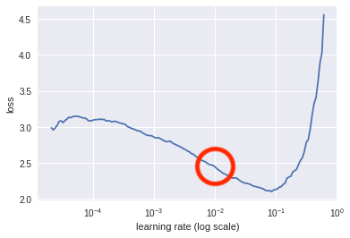
Figure 4-1. Learning rate against loss

In this case, we should look at using a learning rate of around 1e-2 (marked within the circle), as that is roughly the point where the gradient of the descent is steepest.

Note

Note that you’re not looking for the bottom of the curve, which might be the more intuitive place; you’re looking for the point that is getting to the bottom the fastest.

Here’s a simplified version of what the fast.ai library does under the covers:

import math
def find_lr(model, loss_fn, optimizer, init_value=1e-8, final_value=10.0):
    number_in_epoch = len(train_loader) - 1
    update_step = (final_value / init_value) ** (1 / number_in_epoch)
    lr = init_value
    optimizer.param_groups[0]["lr"] = lr
    best_loss = 0.0
    batch_num = 0
    losses = []
    log_lrs = []
    for data in train_loader:
        batch_num += 1
        inputs, labels = data
        inputs, labels = inputs, labels
        optimizer.zero_grad()
        outputs = model(inputs)
        loss = loss_fn(outputs, labels)

        # Crash out if loss explodes

        if batch_num > 1 and loss > 4 * best_loss:
            return log_lrs[10:-5], losses[10:-5]

        # Record the best loss

        if loss < best_loss or batch_num == 1:
            best_loss = loss

        # Store the values

        losses.append(loss)
        log_lrs.append(math.log10(lr))

        # Do the backward pass and optimize

        loss.backward()
        optimizer.step()

        # Update the lr for the next step and store

        lr *= update_step
        optimizer.param_groups[0]["lr"] = lr
    return log_lrs[10:-5], losses[10:-5]

What’s going on here is that we iterate through the batches, training almost as usual; we pass our inputs through the model and then we get the loss from that batch. We record what our best_loss is so far, and compare the new loss against it. If our new loss is more than four times the best_loss, we crash out of the function, returning what we have so far (as the loss is probably tending to infinity). Otherwise, we keep appending the loss and logs of the current learning rate, and update the learning rate with the next step along the way to the maximal rate at the end of the loop. The plot can then be shown using the matplotlib plt function:

logs,losses = find_lr()
plt.plot(logs,losses)
found_lr = 1e-2

Note that we return slices of the lr logs and losses. We do that simply because the first bits of training and the last few (especially if the learning rate becomes very large quite quickly) tend not to tell us much information.

The implementation in fast.ai’s library also includes weighted smoothing, so you get smooth lines in your plot, whereas this snippet produces spiky output. Finally, remember that because this function does actually train the model and messes with the optimizer’s learning rate settings, you should save and reload your model beforehand to get back to the state it was in before you called find_lr() and also reinitialize the optimizer you’ve chosen, which you can do now, passing in the learning rate you’ve determined from looking at the graph!

That gets us a good value for our learning rate, but we can do even better with differential learning rates.

Differential Learning Rates

In our training so far, we have applied one learning rate to the entire model. When training a model from scratch, that probably makes sense, but when it comes to transfer learning, we can normally get a little better accuracy if we try something different: training different groups of layers at different rates. Earlier in the chapter, we froze all the pretrained layers in our model and trained just our new classifier, but we may want to fine-tune some of the layers of, say, the ResNet model we’re using. Perhaps adding some training to the layers just preceding our classifier will make our model just a little more accurate. But as those preceding layers have already been trained on the ImageNet dataset, maybe they need only a little bit of training as compared to our newer layers? PyTorch offers a simple way of making this happen. Let’s modify our optimizer for the ResNet-50 model:

optimizer = optimizer.Adam([
{ 'params': transfer_model.layer4.parameters(), 'lr': found_lr /3},
{ 'params': transfer_model.layer3.parameters(), 'lr': found_lr /9},
], lr=found_lr)

That sets the learning rate for layer4 (just before our classifier) to a third of the found learning rate and a ninth for layer3. That combination has empirically worked out quite well in my work, but obviously feel free to experiment. There’s one more thing, though. As you may remember from the beginning of this chapter, we froze all these pretrained layers. It’s all very well to give them a different learning rate, but as of right now, the model training won’t touch them at all because they don’t accumulate gradients. Let’s change that:

unfreeze_layers = [transfer_model.layer3, transfer_model.layer4]
for layer in unfreeze_layers:
    for param in layer.parameters():
        param.requires_grad = True

Now that the parameters in these layers take gradients once more, the differential learning rates will be applied when you fine-tine the model. Note that you can freeze and unfreeze parts of the model at will and do further fine-tuning on every layer separately if you’d like!

Now that we’ve looked at the learning rates, let’s investigate a different aspect of training our models: the data that we feed into them.

Data Augmentation

One of the dreaded phrases in data science is, Oh no, my model has overfit on the data! As I mentioned in Chapter 2, overfitting occurs when the model decides to reflect the data presented in the training set rather than produce a generalized solution. You’ll often hear people talking about how a particular model memorized the dataset, meaning the model learned the answers and went on to perform poorly on production data.

The traditional way of guarding against this is to amass large quantities of data. By seeing more data, the model gets a more general idea of the problem it is trying to solve. If you view the situation as a compression problem, then if you prevent the model from simply being able to store all the answers (by overwhelming its storage capacity with so much data), it’s forced to compress the input and therefore produce a solution that cannot simply be storing the answers within itself. This is fine, and works well, but say we have only a thousand images and we’re doing transfer learning. What can we do?

One approach that we can use is data augmentation. If we have an image, we can do a number of things to that image that should prevent overfitting and make the model more general. Consider the images of Helvetica the cat in Figures 4-2 and 4-3.

Figure 4-2. Our original image

Figure 4-3. A flipped Helvetica

Obviously to us, they’re the same image. The second one is just a mirrored copy of the first. The tensor representation is going to be different, as the RGB values will be in different places in the 3D image. But it’s still a cat, so the model training on this image will hopefully learn to recognize a cat shape on the left or right side of the frame, rather than simply associating the entire image with cat. Doing this in PyTorch is simple. You may remember this snippet of code from Chapter 2:

transforms = transforms.Compose([
        transforms.Resize(64),
        transforms.ToTensor(),
        transforms.Normalize(mean=[0.485, 0.456, 0.406],
                     std=[0.229, 0.224, 0.225] )
        ])

This forms a transformation pipeline that all images go through as they enter the model for training. But the torchivision.transforms library contains many other transformation functions that can be used to augment training data. Let’s have a look at some of the more useful ones and see what happens to Helvetica with some of the less obvious transforms as well.

Torchvision Transforms

torchvision comes complete with a large collection of potential transforms that can be used for data augmentation, plus two ways of constructing new transformations. In this section, we look at the most useful ones that come supplied as well as a couple of custom transformations that you can use in your own applications.

torchvision.transforms.ColorJitter(brightness=0, contrast=0, saturation=0, hue=0)

ColorJitter randomly changes the brightness, contrast, saturation, and hue of an image. For brightness, contrast, and saturation, you can supply either a float or a tuple of floats, all nonnegative in the range 0 to 1, and the randomness will either be between 0 and the supplied float or it will use the tuple to generate randomness between the supplied pair of floats. For hue, a float or float tuple between –0.5 and 0.5 is required, and it will generate random hue adjustments between [-hue,hue] or [min, max]. See Figure 4-4 for an example.

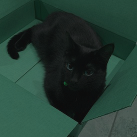
Figure 4-4. ColorJitter applied at 0.5 for all parameters

If you want to flip your image, these two transforms randomly reflect an image on either the horizontal or vertical axis:

torchvision.transforms.RandomHorizontalFlip(p=0.5)
torchvision.transforms.RandomVerticalFlip(p=0.5)

Either supply a float from 0 to 1 for the probability of the reflection to occur or accept the default of a 50% chance of reflection. A vertically flipped cat is shown in Figure 4-5.

Figure 4-5. Vertical flip

RandomGrayscale is a similar type of transformation, except that it randomly turns the image grayscale, depending on the parameter p (the default is 10%):

torchvision.transforms.RandomGrayscale(p=0.1)

RandomCrop and RandomResizeCrop, as you might expect, perform random crops on the image of size, which can either be an int for height and width, or a tuple containing different heights and widths. Figure 4-6 shows an example of a RandomCrop in action.

torchvision.transforms.RandomCrop(size, padding=None,
pad_if_needed=False, fill=0, padding_mode='constant')
torchvision.transforms.RandomResizedCrop(size, scale=(0.08, 1.0),
ratio=(0.75, 1.3333333333333333), interpolation=2)

Now you need to be a little careful here, because if your crops are too small, you run the risk of cutting out important parts of the image and making the model train on the wrong thing. For instance, if a cat is playing on a table in an image, and the crop takes out the cat and just leaves part of the table to be classified as cat, that’s not great. While the RandomResizeCrop will resize the crop to fill the given size, RandomCrop may take a crop close to the edge and into the darkness beyond the image.

Note

RandomResizeCrop is using Bilinear interpolation, but you can also select nearest neighbor or bicubic interpolation by changing the interpolation parameter. See the PIL filters page for further details.

As you saw in Chapter 3, we can add padding to maintain the required size of the image. By default, this is constant padding, which fills out the otherwise empty pixels beyond the image with the value given in fill. However, I recommend that you use the reflect padding instead, as empirically it seems to work a little better than just throwing in empty constant space.

Figure 4-6. RandomCrop with size=100

If you’d like to randomly rotate an image, RandomRotation will vary between [-degrees, degrees] if degrees is a single float or int, or (min,max) if it is a tuple:

torchvision.transforms.RandomRotation(degrees, resample=False,expand=False, center=None)

If expand is set to True, this function will expand the output image so that it can include the entire rotation; by default, it’s set to crop to within the input dimensions. You can specify a PIL resampling filter, and optionally provide an (x,y) tuple for the center of rotation; otherwise the transform will rotate about the center of the image. Figure 4-7 is a RandomRotation transformation with degrees set to 45.

Figure 4-7. RandomRotation with degrees = 45

Pad is a general-purpose padding transform that adds padding (extra height and width) onto the borders of an image:

torchvision.transforms.Pad(padding, fill=0, padding_mode=constant)

A single value in padding will apply padding on that length in all directions. A two-tuple padding will produce padding in the length of (left/right, top/bottom), and a four-tuple will produce padding for (left, top, right, bottom). By default, padding is set to constant mode, which copies the value of fill into the padding slots. The other choices are edge, which pads the last values of the edge of the image into the padding length; reflect, which reflects the values of the image (except the edge) into the border; and symmetric, which is reflection but includes the last value of the image at the edge. Figure 4-8 shows padding set to 25 and padding_mode set to reflect. See how the box repeats at the edges.

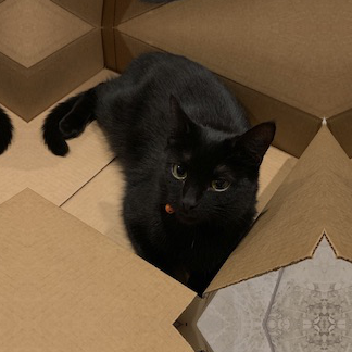
Figure 4-8. Pad with padding = 25 and padding_mode = reflect

RandomAffine allows you to specify random affine translations of the image (scaling, rotations, translations, and/or shearing, or any combination). Figure 4-9 shows an example of an affine transformation.

torchvision.transforms.RandomAffine(degrees, translate=None, scale=None,
shear=None, resample=False, fillcolor=0)

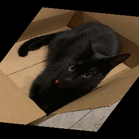
Figure 4-9. RandomAffine with degrees = 10 and shear = 50

The degrees parameter is either a single float or int or a tuple. In single form, it produces random rotations between (–degrees, degrees). With a tuple, it will produce random rotations between (min, max). degrees has to be explicitly set to prevent rotations from occurring—there’s no default setting. translate is a tuple of two multipliers (horizontal_multipler, vertical_multiplier). At transform time, a horizontal shift, dx, is sampled in the range –image_width × horizontal_multiplier < dx < img_width × horizontal_width, and a vertical shift is sampled in the same way with respect to the image height and the vertical multiplier.

Scaling is handled by another tuple, (min, max), and a uniform scaling factor is randomly sampled from those. Shearing can be either a single float/int or a tuple, and randomly samples in the same manner as the degrees parameter. Finally, resample allows you to optionally provide a PIL resampling filter, and fillcolor is an optional int specifying a fill color for areas inside the final image that lie outside the final transform.

As for what transforms you should use in a data augmentation pipeline, I definitely recommend using the various random flips, color jittering, rotation, and crops to start.

Other transformations are available in torchvision; check the documentation for more details. But of course you may find yourself wanting to create a transformation that is particular to your data domain that isn’t included by default, so PyTorch provides various ways of defining custom transformations, as you’ll see next.

Color Spaces and Lambda Transforms

This may seem a little odd to even bring up, but so far all our image work has been in the fairly standard 24-bit RGB color space, where every pixel has an 8-bit red, green, and blue value to indicate the color of that pixel. However, other color spaces are available!

A popular alternative is HSV, which has three 8-bit values for hue, saturation, and value. Some people feel this system more accurately models human vision than the traditional RGB color space. But why does this matter? A mountain in RGB is a mountain in HSV, right?

Well, there’s some evidence from recent deep learning work in colorization that other color spaces can produce slightly higher accuracy than RGB. A mountain may be a mountain, but the tensor that gets formed in each space’s representation will be different, and one space may capture something about your data better than another.

When combined with ensembles, you could easily create a series of models that combines the results of training on RGB, HSV, YUV, and LAB color spaces to wring out a few more percentage points of accuracy from your prediction pipeline.

One slight problem is that PyTorch doesn’t offer a transform that can do this. But it does provide a couple of tools that we can use to randomly change an image from standard RGB into HSV (or another color space). First, if we look in the PIL documentation, we see that we can use Image.convert() to translate a PIL image from one color space to another. We could write a custom transform class to carry out this conversion, but PyTorch adds a transforms.Lambda class so that we can easily wrap any function and make it available to the transform pipeline. Here’s our custom function:

def _random_colour_space(x):
    output = x.convert("HSV")
    return output

This is then wrapped in a transforms.Lambda class and can be used in any standard transformation pipeline like we’ve seen before:

colour_transform = transforms.Lambda(lambda x: _random_colour_space(x))

That’s fine if we want to convert every image into HSV, but really we don’t want that. We’d like it to randomly change images in each batch, so it’s probable that the image will be presented in different color spaces in different epochs. We could update our original function to generate a random number and use that to generate a random probability of changing the image, but instead we’re even lazier and use RandomApply:

random_colour_transform = torchvision.transforms.RandomApply([colour_transform])

By default, RandomApply fills in a parameter p with a value of 0.5, so there’s a 50/50 chance of the transform being applied. Experiment with adding more color spaces and the probability of applying the transformation to see what effect it has on our cat and fish problem.

Let’s look at another custom transform that is a little more complicated.

Custom Transform Classes

Sometimes a simple lambda isn’t enough; maybe we have some initialization or state that we want to keep track of, for example. In these cases, we can create a custom transform that operates on either PIL image data or a tensor. Such a class has to implement two methods: __call__, which the transform pipeline will invoke during the transformation process; and __repr__, which should return a string representation of the transform, along with any state that may be useful for diagnostic purposes.

In the following code, we implement a transform class that adds random Gaussian noise to a tensor. When the class is initialized, we pass in the mean and standard distribution of the noise we require, and during the __call__ method, we sample from this distribution and add it to the incoming tensor:

class Noise():
    """Adds gaussian noise to a tensor.

        >>> transforms.Compose([
        >>>     transforms.ToTensor(),
        >>>     Noise(0.1, 0.05)),
        >>> ])

    """
    def __init__(self, mean, stddev):
        self.mean = mean
        self.stddev = stddev

    def __call__(self, tensor):
        noise = torch.zeros_like(tensor).normal_(self.mean, self.stddev)
        return tensor.add_(noise)

    def __repr__(self):
        repr = f"{self.__class__.__name__  }(mean={self.mean},
               stddev={self.stddev})"
        return repr

If we add this to a pipeline, we can see the results of the __repr__ method being called:

transforms.Compose([Noise(0.1, 0.05))])
>> Compose(
    Noise(mean=0.1,sttdev=0.05)
)

Because transforms don’t have any restrictions and just inherit from the base Python object class, you can do anything. Want to completely replace an image at runtime with something from Google image search? Run the image through a completely different neural network and pass that result down the pipeline? Apply a series of image transforms that turn the image into a crazed reflective shadow of its former self? All possible, if not entirely recommended. Although it would be interesting to see whether Photoshop’s Twirl transformation effect would make accuracy worse or better! Why not give it a go?

Aside from transformations, there are a few more ways of squeezing as much performance from a model as possible. Let’s look at more examples.

Start Small and Get Bigger!

Here’s a tip that seems odd, but obtains real results: start small and get bigger. What I mean is if you’re training on 256 × 256 images, create a few more datasets in which the images have been scaled to 64 × 64 and 128 × 128. Create your model with the 64 × 64 dataset, fine-tune as normal, and then train the exact same model with the 128 × 128 dataset. Not from scratch, but using the parameters that have already been trained. Once it looks like you’ve squeezed the most out of the 128 × 128 data, move on to your target 256 × 256 data. You’ll probably find a percentage point or two improvement in accuracy.

While we don’t know exactly why this works, the working theory is that by training at the lower resolutions, the model learns about the overall structure of the image and can refine that knowledge as the incoming images expand. But that’s just a theory. However, that doesn’t stop it from being a good little trick to have up your sleeve when you need to squeeze every last bit of performance from a model.

If you don’t want to have multiple copies of a dataset hanging around in storage, you can use torchvision transforms to do this on the fly using the Resize function:

resize = transforms.Compose([ transforms.Resize(64),
 …_other augmentation transforms_…
 transforms.ToTensor(),
 transforms.Normalize([0.485, 0.456, 0.406], [0.229, 0.224, 0.225])

The penalty you pay here is that you end up spending more time in training, as PyTorch has to apply the resize every time. If you resized all the images beforehand, you’d likely get a quicker training run, at the expense of filling up your hard drive. But isn’t that trade-off always the way?

The concept of starting small and then getting bigger also applies to architectures. Using a ResNet architecture like ResNet-18 or ResNet-34 to test out approaches to transforms and get a feel for how training is working provides a much tighter feedback loop than if you start out using a ResNet-101 or ResNet-152 model. Start small, build upward, and you can potentially reuse the smaller model runs at prediction time by adding them to an ensemble model.

Ensembles

What’s better than one model making predictions? Well, how about a bunch of them? Ensembling is a technique that is fairly common in more traditional machine learning methods, and it works rather well in deep learning too. The idea is to obtain a prediction from a series of models, and combine those predictions to produce a final answer. Because different models will have different strengths in different areas, hopefully a combination of all their predictions will produce a more accurate result than one model alone.

There are plenty of approaches to ensembles, and we won’t go into all of them here. Instead, here’s a simple way of getting started with ensembles, one that has eeked out another 1% of accuracy in my experience; simply average the predictions:

# Assuming you have a list of models in models, and input is your input tensor

predictions = [m[i].fit(input) for i in models]
avg_prediction = torch.stack(b).mean(0).argmax()

The stack method concatenates the array of tensors together, so if we were working on the cat/fish problem and had four models in our ensemble, we’d end up with a 4 × 2 tensor constructed from the four 1 × 2 tensors. And mean does what you’d expect, taking the average, although we have to pass in a dimension of 0 to ensure that it takes an average across the first dimension instead of simply adding up all the tensor elements and producing a scalar output. Finally, argmax picks out the tensor index with the highest element, as you’ve seen before.

It’s easy to imagine more complex approaches. Perhaps weights could be added to each individual model’s prediction, and those weights adjusted if a model gets an answer right or wrong. What models should you use? I’ve found that a combination of ResNets (e.g., 34, 50, 101) work quite well, and there’s nothing to stop you from saving your model regularly and using different snapshots of the model across time in your ensemble!

Conclusion

As we come to the end of Chapter 4, we’re leaving images behind to move on to text. Hopefully you not only understand how convolutional neural networks work on images, but also have a deep bag of tricks in hand, including transfer learning, learning rate finding, data augmentation, and ensembling, which you can bring to bear on your particular application domain.

Further Reading

If you’re interested in learning more in the image realm, check out the fast.ai course by Jeremy Howard, Rachel Thomas, and Sylvain Gugger. This chapter’s learning rate finder is, as I mentioned, a simplified version of the one they use, but the course goes into further detail about many of the techniques in this chapter. The fast.ai library, built on PyTorch, allows you to bring them to bear on your image (and text!) domains easily.

• Torchvision documentation

• PIL/Pillow documentation

• “Cyclical Learning Rates for Training Neural Networks” by Leslie N. Smith (2015)

• “ColorNet: Investigating the Importance of Color Spaces for Image Classification” by Shreyank N. Gowda and Chun Yuan (2019)

¹ See “Cyclical Learning Rates for Training Neural Networks” by Leslie Smith (2015).