Programming Quantum Computers

Chapter 4. Quantum Teleportation

In this chapter we introduce a QPU program allowing us to immediately teleport an object across a distance of 3.1 millimeters! The same code would work over interstellar distances, given the right equipment.

Although teleportation might conjure up images of magician’s parlor tricks, we’ll see that the kind of quantum teleportation we can perform with a QPU is equally impressive, yet far more practical—and is, in fact, an essential conceptual component of QPU programming.

Hands-on: Let’s Teleport Something

The best way to learn about teleportation is to try to do it. Keep in mind that throughout all of human history up until the time of writing, only a few thousand people have actually performed physical teleportation of any kind, so just running the following code makes you a pioneer.

For this example, rather than a simulator, we will use IBM’s five-qubit actual QPU, as seen in Figure 4-1. You’ll be able to paste the sample code from Example 4-1 into the IBM Q Experience website, click a button, and confirm that your teleportation was successful.

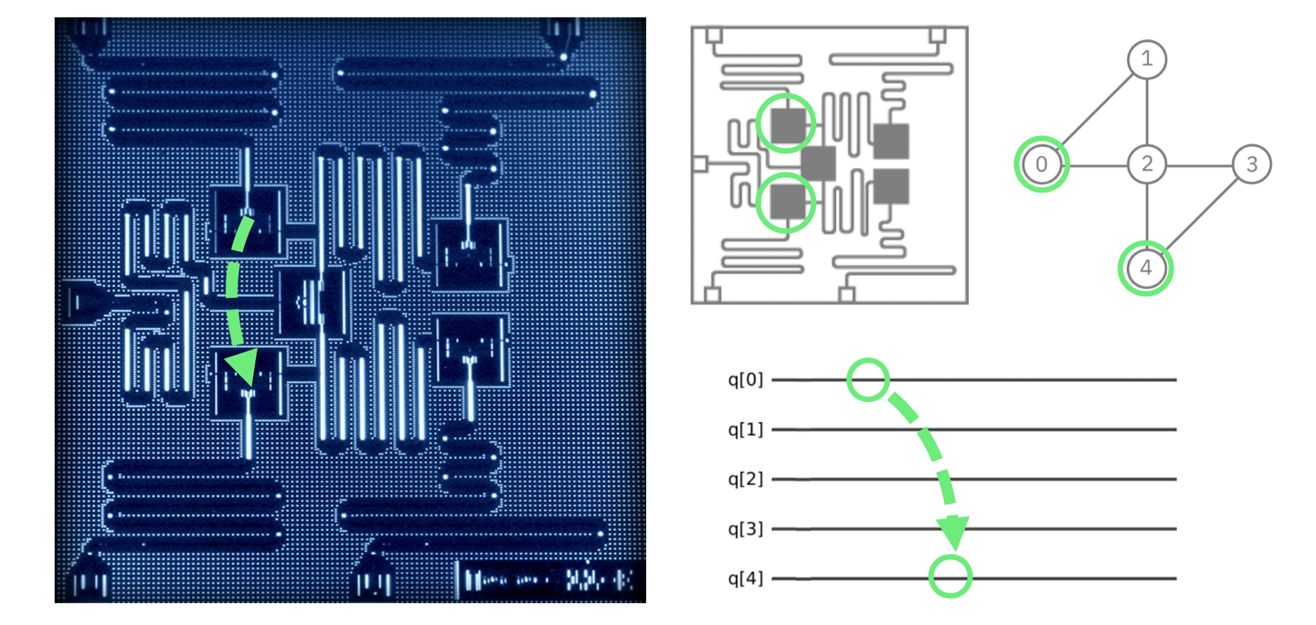
Figure 4-1. The IBM chip is very small, so the qubit does not have far to go; the image and schematics show the regions on the QPU we will teleport between¹

The IBM Q Experience can be programmed using OpenQASM,² and also Qiskit.³ Note that the code in Example 4-1 is not JavaScript to be run on QCEngine, but rather OpenQASM code to be run online through IBM’s cloud interface, shown in Figure 4-2. Doing so allows you to not just simulate, but actually perform the teleportation of a qubit currently at IBM’s research center in Yorktown Heights, New York. We’ll walk you through how to do this. Following through the code in detail will also help you understand precisely how quantum teleportation works.

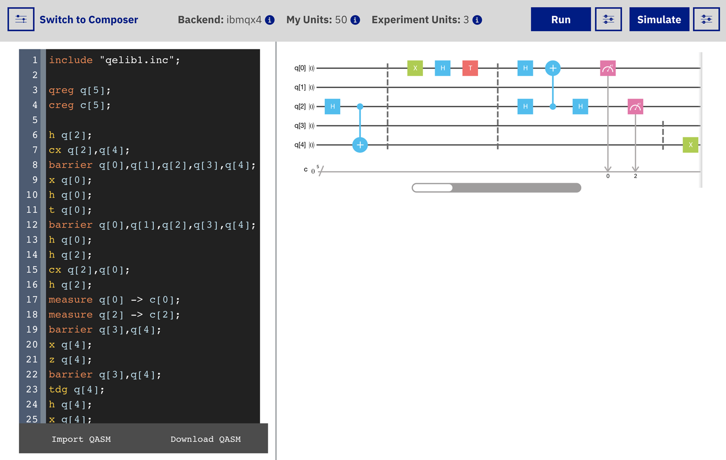
Figure 4-2. The IBM Q Experience (QX) OpenQASM online editor⁴

Sample Code

Run this sample online at http://oreilly-qc.github.io?p=4-1.

Example 4-1. Teleport and verify

include "qelib1.inc";
qreg q[5];
creg c[5];

// Step 1: Create an entangled pair
h q[2];
cx q[2],q[4];
barrier q[0],q[1],q[2],q[3],q[4];

// Step 2: Prepare a payload
x q[0];
h q[0];
t q[0];
barrier q[0],q[1],q[2],q[3],q[4];

// Step 3: Send
h q[0];
h q[2];
cx q[2],q[0];
h q[2];
measure q[0] -> c[0];
measure q[2] -> c[2];
barrier q[3],q[4];

// Step 4: Receive
x q[4];
z q[4];
barrier q[3],q[4];

// Step 5: Verify
tdg q[4];
h q[4];
x q[4];
measure q[4] -> c[4];

Before getting to the details, first some clarifying points. By quantum teleportation we mean the ability to transport the precise state (i.e., magnitudes and relative phase) of one qubit to another. Our intention is to take all the information contained in the first qubit and put it in the second qubit. Recall that quantum information cannot be replicated; hence the information on the first qubit is necessarily destroyed when we teleport it to the second one. Since a quantum description is the most complete description of a physical object, this is actually precisely what you might colloquially think of as teleportation—only at the quantum level.⁵

With that out of the way, let’s teleport! The textbook introduction to quantum teleportation begins with a story that goes something like this: A pair of qubits in an entangled state are shared between two parties, Alice and Bob (physicists have an obsession with anthropomorphizing the alphabet). These entangled qubits are a resource that Alice will use to teleport the state of some other qubit to Bob. So teleportation involves three qubits: the payload qubit that Alice wants to teleport, and an entangled pair of qubits that she shares with Bob (and that acts a bit like a quantum Ethernet cable). Alice prepares her payload and then, using HAD and CNOT operations, she entangles this payload qubit with her other qubit (which is, in turn, already entangled with Bob’s qubit). She then destroys both her payload and the entangled qubit using READ operations. The results from these READ operations yield two conventional bits of information that she sends to Bob. Since these are bits, rather than qubits, she can use a conventional Ethernet cable for this part. Using those two bits, Bob performs some single-qubit operations on his half of the entangled pair originally shared with Alice, and lo and behold, it becomes the payload qubit that Alice intended to send.

Before we walk through the detailed protocol of quantum operations described here,⁶ you may have a concern in need of addressing. “Hang on…” (we imagine you saying), “if Alice is sending Bob conventional information through an Ethernet cable…” (you continue), “then surely this isn’t that impressive at all.” Excellent observation! It is certainly true that quantum teleportation crucially relies on the transmission of conventional (digital) bits for its success. We’ve already seen that the magnitudes and relative phases needed to fully describe an arbitrary qubit state can take on a continuum of values. Crucially, the teleportation protocol works even in the case when Alice does not know the state of her qubit. This is particularly important since it is impossible to determine the magnitude and relative phase of a single qubit in an unknown state. And yet—with the help of an entangled pair of qubits—only two conventional bits were needed to effectively transmit the precise configuration of Alice’s qubit (whatever its amplitudes were). This configuration will be correct to a potentially infinite number of bits of precision!

So how do we engineer this magic? Here’s the full protocol. Figure 4-3 shows the operations that we must employ on the three involved qubits. All these operations were introduced in Chapters 2 and 3.

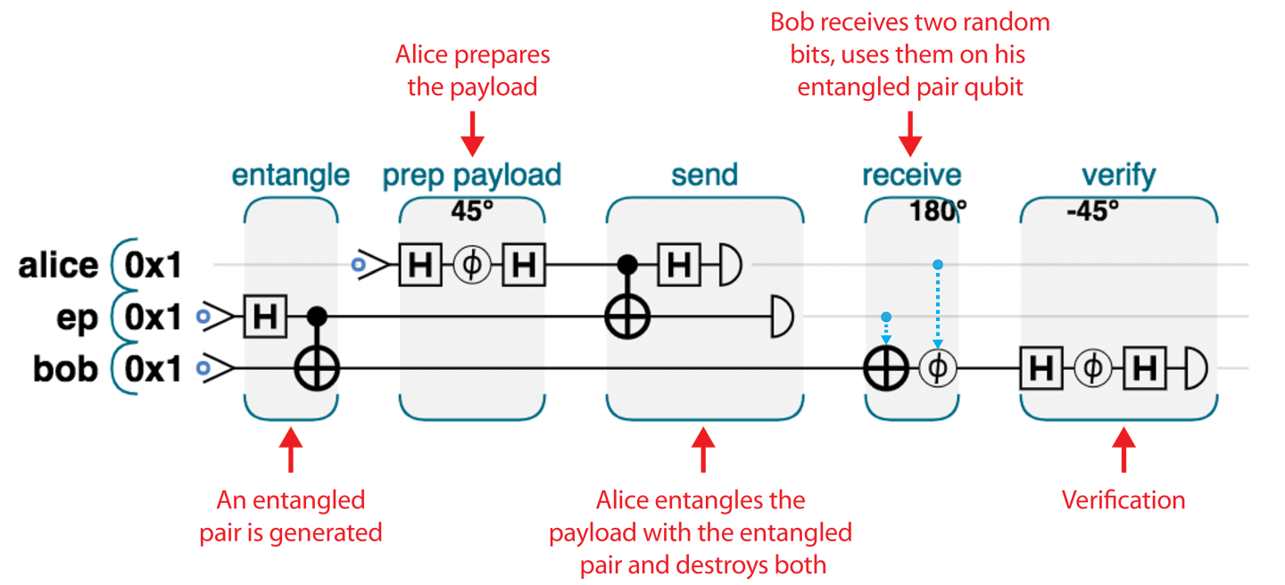
Figure 4-3. Complete teleportation circut: Alice holds the alice and ep qubits, while Bob holds bob

If you paste the code for this circuit from Example 4-1 into the IBM QX system, the IBM user interface will display the circuit shown in Figure 4-4. Note that this is exactly the same program as we’ve shown in Figure 4-3, just displayed slightly differently. The quantum gate notation we’ve been using is standardized, so you can expect to find it used outside this book.⁷

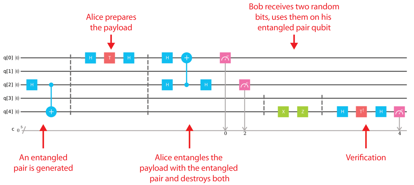
Figure 4-4. Teleportation circuit in IBM QX⁸

When you click Run, IBM will run your program 1,024 times (this number is adjustable) and then display statistics regarding all of these runs. After running the program, you can expect to find something similar (although not identical) to the bar chart shown in Figure 4-5.

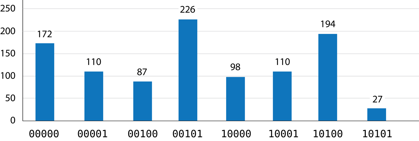
Figure 4-5. Results of running the program (teleportation success?)

Success? Maybe! To demonstrate how to read and interpret these results, let’s walk through each step in the QPU program in a little more detail, using circle notation to visualize what’s happening to our qubits.⁹

Tip

At the time of writing, the circuits and results displayed by IBM QX show what’s happening with all five qubits available in the QPU, even if we’re not using them all. This is why there are two empty qubit lines in the circuit shown in Figure 4-4, and why the bars showing results for each output in Figure 4-5 are labeled with a five-bit (rather than three-bit) binary number—even though only the bars corresponding to the 2³ = 8 possible configurations of the three qubits we used are actually shown.

Program Walkthrough

Since we use three qubits in our teleportation example, their full description needs 2³ = 8 circles (one for each possible combination of the 3 bits). We’ll arrange these eight circles in two rows, which helps us to visualize how operations affect the three constituent qubits. In Figure 4-6 we’ve labeled each row and column of circles corresponding to a given qubit having a particular value. You can check that these labels are correct by considering the binary value of the register that each circle corresponds to.

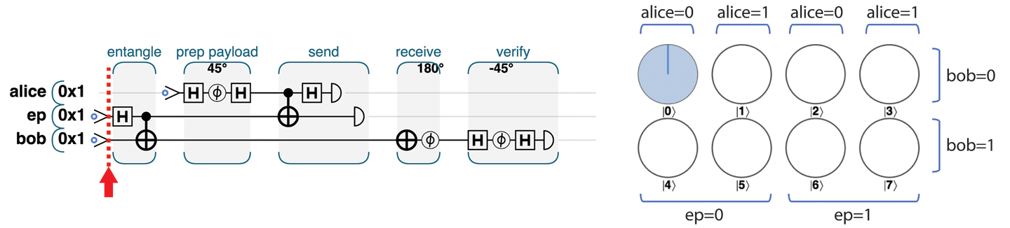
Figure 4-6. The complete teleport-and-verify program

Note

When dealing with multi-qubit registers we’ll often arrange our circle notation in rows and columns as we do in Figure 4-6. This is always a useful way of more quickly spotting the behavior of individual qubits: it’s easy to pick out the relevant rows or columns.

At the beginning of the program, all three qubits are initialized in state ∣0⟩, as indicated in Figure 4-6—the only possible value is the one where alice=0 and ep=0 and bob=0.

Step 1: Create an Entangled Pair

The first task for teleportation is establishing an entangled link. The HAD and CNOT combination achieving this is the same process we used in Chapter 3 to create the specially named Bell pair entangled state of two qubits. We can readily see from the circle notation in Figure 4-7 that if we read bob and ep, the values are 50/50 random, but guaranteed to match each other, à la entanglement.

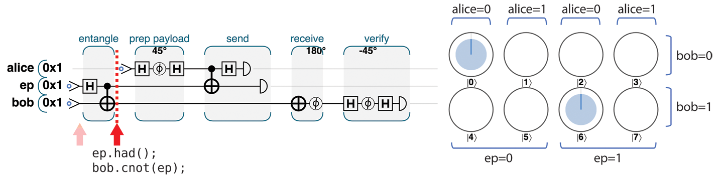
Figure 4-7. Step 1: Create an entangled pair

Step 2: Prepare the Payload

Having established an entanglement link, Alice can prepare the payload to be sent. How she prepares it depends, of course, on the nature of the (quantum) information that she wants to send to Bob. She might write a value to the payload qubit, entangle it with some other QPU data, or even receive it from a previous computation in some entirely separate part of her QPU.

For our example here we’ll disappoint Alice by asking her to prepare a particularly simple payload qubit, using only HAD and PHASE operations. This has the benefit of producing a payload with a readily decipherable circle-notation pattern, as shown in Figure 4-8.

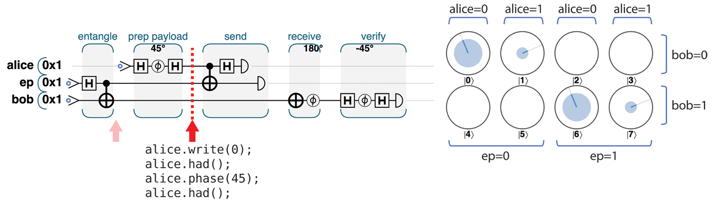
Figure 4-8. Step 2: Prepare the payload

We can see that the bob and ep qubits are still dependent on one another (only the circles corresponding to the bob and ep qubits possessing equal values have nonzero magnitudes). We can also see that the value of alice is not dependent on either of the other two qubits, and furthermore that her payload preparation produced a qubit that is 85.4% ∣0⟩ and 14.6% ∣1⟩, with a relative phase of –90° (the circles corresponding to alice=1 are at 90° clockwise of the alice=0 circles, which is negative in our convention).

Step 3.1: Link the Payload to the Entangled Pair

In Chapter 2 we saw that the conditional nature of the CNOT operation can entangle the states of two qubits. Alice now uses this fact to entangle her payload qubit with her half of the entangled pair she already shares with Bob. In terms of circle notation, this action swaps circles around as shown in Figure 4-9.

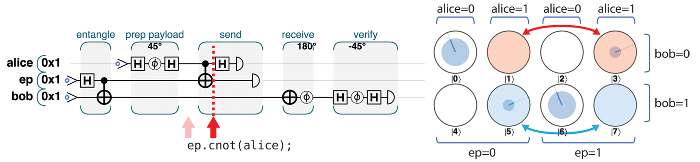
Figure 4-9. Step 3.1: Link the payload to the entangled pair

Now that we have multiple entangled states, there’s the potential for a little confusion—so let’s be clear. Alice and Bob already each held one of two entangled qubits (produced in step 1). Now Alice has entangled another (payload) qubit onto her half of this (already entangled) pair. Intuitively we can see that in some sense Alice has, by proxy, now linked her payload to Bob’s half of the entangled pair—although her payload qubit is still unchanged. READ results on her payload will now be logically linked with those of the other two qubits. We can see this link in circle notation since the QPU register state in Figure 4-9 only contains entries where the XOR of all three qubits is 0. Formerly this was true of ep and bob, but now it is true for all three qubits forming a three-qubit entangled group.

Step 3.2: Put the Payload into a Superposition

To make the link that Alice has created for her payload actually useful, she needs to finish by performing a HAD operation on her payload, as shown in Figure 4-10.

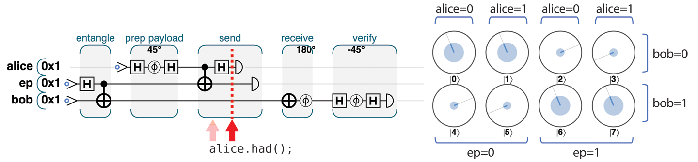
Figure 4-10. Step 3.2: Put the payload into a superposition

To see why Alice needed this HAD, take a look at the circle-notation representation of the state of the three qubits shown in Figure 4-10. In each column there is a pair of circles, showing a qubit that Bob might receive (we’ll see shortly that precisely which one he would receive depends on the results of the READs that Alice performs). Interestingly, the four potential states Bob could receive are all different variations on Alice’s original payload:

• In the first column (where alice=0 and ep=0), we have Alice’s payload, exactly as she prepared it.

• In the second column, we have the same thing, except with a PHASE(180) applied.

• In the third column, we see the correct payload, but with a NOT having been applied to it (∣0⟩ and ∣1⟩ are flipped).

• Finally, the last column is both phase-shifted and flipped (i.e., a PHASE(180) followed by a NOT).

If Alice hadn’t applied HAD, she would have destroyed magnitude and phase information when applying her READ operations that she will shortly use (try it!). By applying the HAD operation, Alice was able to maneuver the state of Bob’s qubit closer to that of her payload.

Step 3.3: READ Both of Alice’s Qubits

Next, Alice performs a READ operation on her two qubits (the payload and her half of the entangled pair she shares with Bob). This READ irrevocably destroys both these qubits. You may wonder why Alice bothers to do this. As we’ll see, it turns out that the results of this unavoidably destructive READ operation are crucial for the teleportation protocol to work. Copying quantum states is not possible, even when using entanglement. The only option to communicate quantum states is to teleport them, and when teleporting, we must destroy the original.

In Figure 4-11, Alice performs the prescribed READ operations on her payload and her half of the entangled pair. This operation returns two bits.

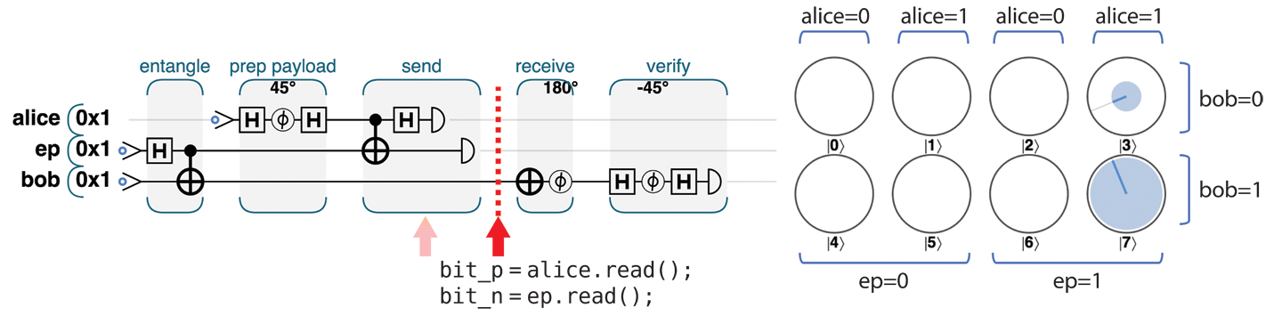
Figure 4-11. Step 3.3: READ both of Alice’s qubits

In terms of circle notation, Figure 4-11 shows that by reading the values of her qubits Alice has selected one column of circles (which one she gets being dependent on the random READ results), resulting in the circles outside this column having zero magnitude.

Step 4: Receive and Transform

In “Step 3.2: Put the Payload into a Superposition” we saw that Bob’s qubit could end up in one of four states—each of which is simply related to Alice’s payload by HAD and/or PHASE(180) operations. If Bob could learn which of these four states he possessed, he could apply the necessary inverse operations to convert it back to Alice’s original payload. And the two bits Alice has from her READ operations are precisely the information that Bob needs! So at this stage, Alice picks up the phone and transmits two bits of conventional information to Bob.

Based on which two bits he receives, Bob knows which column from our circle-notation view represents his qubit. If the first bit he receives from Alice is 1, he performs a NOT operation on the qubit. Then, if the second bit is 1 he also performs a PHASE(180), as illustrated in Figure 4-12.

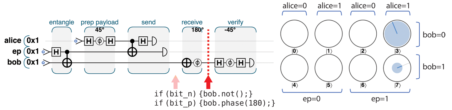
Figure 4-12. Step 4: Receive and transform

This completes the teleportation protocol—Bob now holds a qubit indistinguishable from Alice’s initial payload.

Note

The current IBM QX hardware does not support the kind of feed-forward operation we need to allow the (completely random) bits from Alice’s READ to control Bob’s actions. This shortcoming can be circumvented by using post-selection—we have Bob perform the same operation no matter what Alice sends. This behavior may exasperate Alice, as shown in Figure 4-13. Then we look at all of the outputs, and discard all but the results where Bob did what he would have with the benefit of information from Alice.

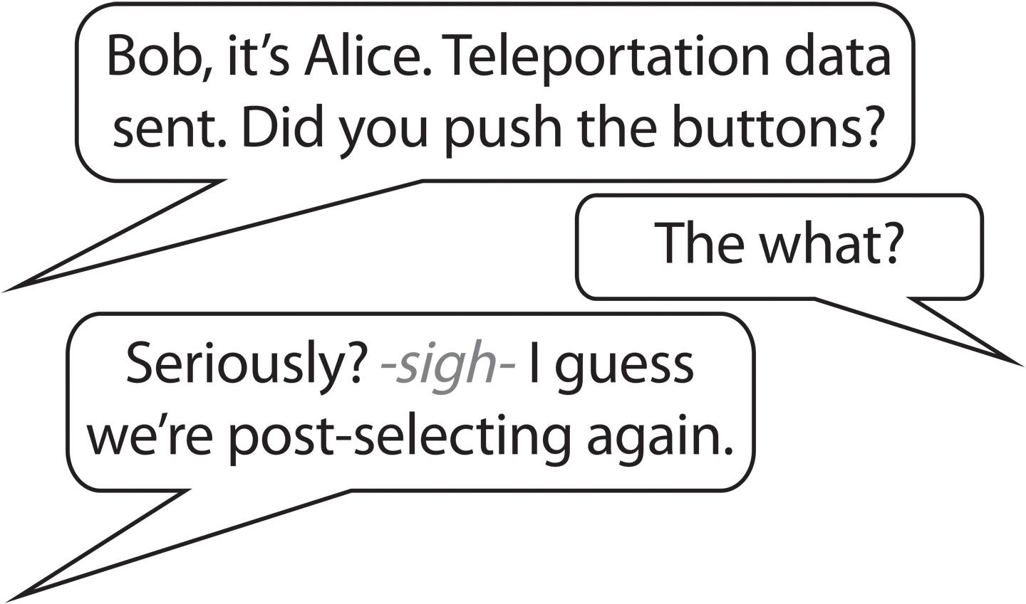
Figure 4-13. Instead of feed-forward, we can assume Bob is asleep at the switch and throw away cases where he makes wrong decisions

Step 5: Verify the Result

If Alice and Bob were using this teleportation in serious work, they’d be finished. Bob would take the teleported qubit from Alice and continue to use it in whatever larger quantum application they were working on. So long as they trust their QPU hardware, they can rest assured that Bob has the qubit Alice intended.

But, what about cases where we’d like to verify that the hardware has teleported a qubit correctly (even if we don’t mind destroying the teleported qubit in the process)? Our only option is to READ Bob’s final qubit. Of course, we can never expect to learn (and therefore verify) the state of his qubit from a single READ, but by repeating the whole teleportation process and doing multiple READs we can start to build up a picture of Bob’s state.

In fact, the easiest way for us to verify the teleportation protocol’s success on a physical device would be for Bob to run the “prep the payload” steps that Alice performs on a ∣0⟩ state to create her payload, on his final qubit, only in reverse. If the qubit Bob has truly matches the one Alice sent, this should leave Bob with a ∣0⟩ state, and if Bob then performs a final verification READ, it should only ever return a 0. If Bob ever READs this test qubit as nonzero, the teleportation has failed. This additional step for verification is shown in Figure 4-14.

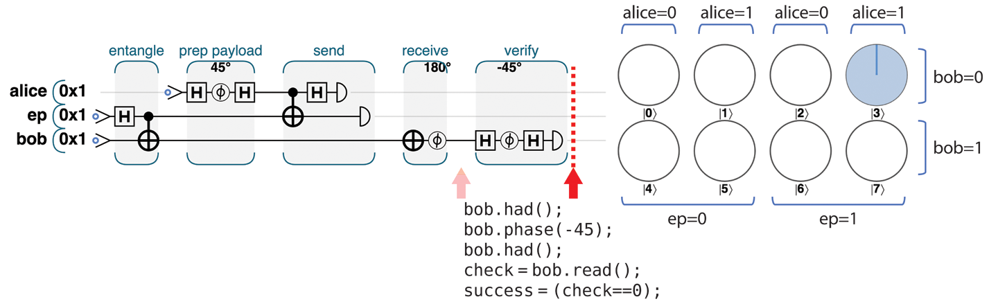
Figure 4-14. Step 5: Verify the result

Even if Alice and Bob are doing serious teleporter work, they will probably want to intersperse their actual teleportations with many verification tests such as these, just to be reassured that their QPU is working correctly.

Interpreting the Results

Armed with this fuller understanding of the teleportation protocol and its subtleties, let’s return to the results obtained from our physical teleportation experiment on the IBM QX. We now have the necessary knowledge to decode them.

There are three READ operations performed in the entire protocol: two by Alice as part of the teleportation, and one by Bob for verification purposes. The bar chart in Figure 4-5 enumerates the number of times each of the 8 possible combinations of these outcomes occurred during 1,024 teleportation attempts.

As noted earlier, we’ll be post-selecting on the IBM QX for instances where Bob happens to perform the right operations (as if he had acted on Alice’s READ results). In the example circuit we gave the IBM QX in Figure 4-4, Bob always performs both a HAD and a PHASE(180) on his qubit, so we need to post-select on cases where Alice’s two READ operations gave 11. This leaves two sets of actually useful results where Bob’s actions happened to correctly match up with Alice’s READ results, as shown in Figure 4-15.

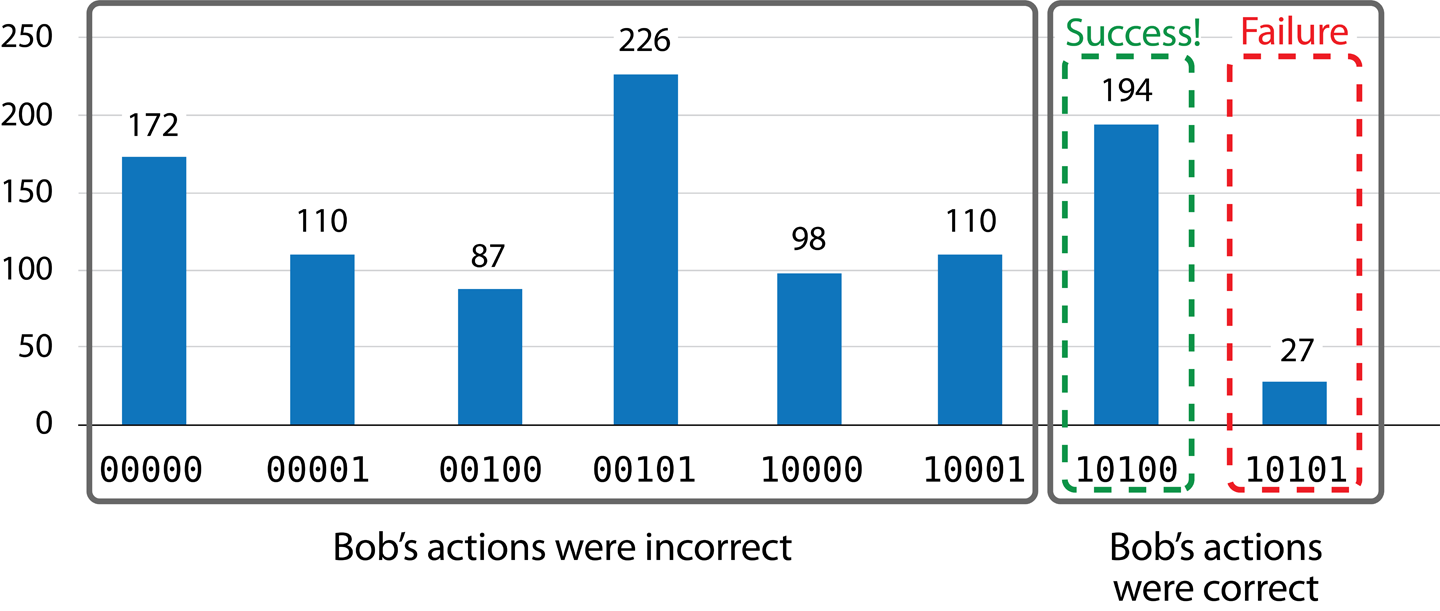
Figure 4-15. Interpreted teleportation results

Of the 221 times where Bob did the correct thing, the teleportation succeeded when Bob’s verification READ gave a value of 0 (since he uses the verification step we discussed previously). This means the teleportation succeeded 194 times, and failed 27 times. A success rate of 87.8% is not bad, considering Alice and Bob are using the best available equipment in 2019. Still, they may think twice before sending anything important.

Warning

If Bob receives an erroneously teleported qubit that is almost like the one Alice sent, the verification is likely to report success. Only by running this test many times can we gain confidence that the device is working well.

How Is Teleportation Actually Used?

Teleportation is a surprisingly fundamental part of the operation of a QPU—even in straight computational applications that have no obvious “communication” aspect at all. It allows us to shuttle information between qubits while working around the “no-copying” constraint. In fact, most practical uses of teleportation are over very short distances within a QPU as an integral part of quantum applications. In the upcoming chapters, you’ll see that most quantum operations for two or more qubits function by forming various types of entanglement. The use of such quantum links to perform computation can usually be seen as an application of the general concept of teleportation. Though we may not explicitly acknowledge teleportation in the algorithms and applications we cover, it plays a fundamental role.

Fun with Famous Teleporter Accidents

As science fiction enthusiasts, our personal favorite use of teleportation is the classic film The Fly. Both the 1958 original and the more modern 1986 Jeff Goldblum version feature an error-prone teleportation experiment. After the protagonist’s cat fails to teleport correctly, he decides that the next logical step is to try it himself, but without his knowledge a fly has gotten into the chamber with him.

We feel a little guilty for bringing the crushing news that actual quantum teleportation doesn’t live up to what’s promised in The Fly. To try to make it up to you, we’ve put together some sample code to teleport a quantum image of a fly—even including the small amount of error called for in the movie’s plot. The code sample can be run online at http://oreilly-qc.github.io?p=4-2, and the horrifying result it produces is shown in Figure 4-16.

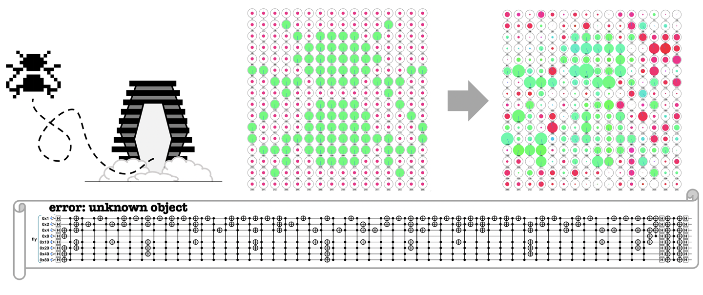
Figure 4-16. Be afraid. Be very afraid.

¹ Courtesy of International Business Machines Corporation, © International Business Machines Corporation.

² OpenQASM is the quantum assembly language supported by IBM Q Experience.

³ Qiskit is an open-source software development kit for working with the IBM Q quantum processors.

⁴ Courtesy of International Business Machines Corporation, © International Business Machines Corporation.

⁵ The caveat, of course, is that humans are made up of many, many quantum states, and so teleporting qubit states is far removed from any idea of teleportation as a mode of transportation. In other words, although teleportation is an accurate description, Lt. Reginald Barclay doesn’t have anything to worry about just yet.

⁶ The complete source code for both the QASM and QCEngine versions of this example can be seen at http://oreilly-qc.github.io?p=4-1.

⁷ Gates such as CNOTs and HADs can be combined in different ways to produce the same result. Some operations have different decompositions in IBM QX and QCEngine.

⁸ Courtesy of International Business Machines Corporation, © International Business Machines Corporation.

⁹ The complete source code for this example can be seen at http://oreilly-qc.github.io?p=4-1.