Chapter 7. Graph Data in the Real World
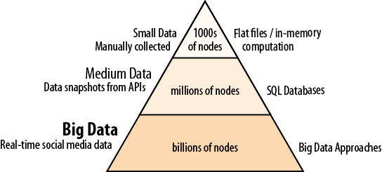
So far we have been dealing with fairly simple datasets, in flat files. Flat files are great for quick analysis: they are portable and mostly human-readable, not to mention accessible to UNIX powertools. This convenience, however, fades quickly when our involvement with the data broadens, as we show in Figure 7-1.

NetworkX is a spectacular tool, with one important limitation: memory. The graph we want to study has to fit entirely in memory. To put this in perspective, a mostly connected graph of 1,000 nodes (binomial, connection probability 0.8 = 800,000 edges) uses 100MB of memory, without any attributes. The same graph with 2,000 nodes (and almost 2 million edges) uses 500MB. In general, memory usage is bounded by O(n)=n+n2=n(n+1). One can easily find this out firsthand by creating a graph in an interactive Python session and observing its memory usage.
Note
Until the late 1990s, social network data has been gathered and compiled manually. The ways to gather data included surveys, psychology experiments, and working with large amounts of text (“text coding”) to extract nodes and relationships. As a result, gathering a dataset of a few hundred nodes was considered a monumental effort worthy of a Ph.D.; there was simply no need to handle larger datasets.
Now, suppose we were scientifically curious about what goes ...
Get Social Network Analysis for Startups now with the O’Reilly learning platform.
O’Reilly members experience books, live events, courses curated by job role, and more from O’Reilly and nearly 200 top publishers.

