Statistical and Machine Learning Approaches for Network Analysis

6.3 A Simple Worked Example

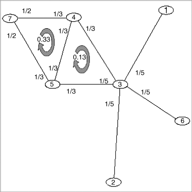
After the fairly theoretical previous section, we aim at giving the reader a better intuition behind the WSD with a simple example. Figure 6.2 shows a small network, called G₁, with seven nodes and eight links. As can be seen there are two cycles of length 3 in this network and one of length 4. We will take N = 3 in this example for convenience and without loss of generality. The random walk probabilities are labeled in Figure 6.2. For example, node 3 has a degree of 5 resulting in a probability of 1/5 th for each edge. The total probability of taking a random walk around each 3-cycle is 6 × 1/2 × 1/3 × 1/3 = 0.33, also shown in Figure.⁶

Figure 6.2 A simple example network G₁.

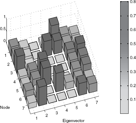
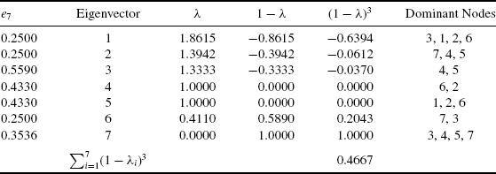
Figure 6.3 shows a 3D plot of the absolute value (for clarity) of the eigenvectors of the normalized Laplacian. The corresponding eigenvalues are shown in Table 6.1.

Figure 6.3 Eigenvectors of the simple example network.

Table 6.1 Eigenvalues, WSD, and Dominant Nodes of Example Network.

The eigenvectors of the normalized Laplacian can be used to form a partitioning of the nodes in a graph. In this example, nodes 4 and 5 are grouped into eigenvector 3, nodes 1, 2, and 6 into eigenvectors ...