Time Series Databases: New Ways to Store and Access Data

Chapter 4. Practical Time Series Tools

“In theory, theory and practice are the same. In practice, they are not.”

—Albert Einstein

As valuable as theory is, practice matters more. Chapter 3 described the theory behind high-performance time series databases leading up to the hybrid and direct-insertion blob architecture that allows very high ingest and analysis rates. This chapter describes how that theory can be implemented using open source software. The open source tools described in this chapter mainly comprise those listed in Table 4-1.

Table 4-1. Open source tools useful for preparing, loading, and accessing data in high-performance NoSQL time series databases.

Open Source Tool	Author	Purpose
Open TSDB	Benoit Sigoure (originally)	Collect, process, and load time series data into storage tier
Extensions to Open TSDB	MapR Technologies	Enable direct blog insertion
Grafana	Torkel Ödegaard and Coding Instinct AB	User interface for accessing and visualizing time series data

We also show how to analyze Open TSDB time series data using open source tools such as R and Apache Spark. At the end of this chapter, we describe how you can attach Grafana, an open source dashboarding tool, to Open TSDB to make it much more useful.

Introduction to Open TSDB: Benefits and Limitations

Originally just for systems monitoring, Open TSDB has proved far more versatile and useful than might have been imagined originally. Part of this versatility and longevity is due to the fact that the underlying storage engine, based on either Apache HBase or MapR-DB, allows a high degree of schema flexibility. The Open TSDB developers have used this to their advantage by starting with something like a star schema design, moving almost immediately to a wide table design, and later extending it with a compressor function to convert wide rows into blobs. (The concepts behind these approaches was explained in Chapter 3.) As the blob architecture was introduced, the default time window was increased from the original 60 seconds to a more blob-friendly one hour in length.

As it stands, however, Open TSDB also suffers a bit from its history and will not support extremely high data rates. This limitation is largely caused by the fact that data is only compacted into the performance-friendly blob format after it has already been inserted into the database in the performance-unfriendly wide table format.

The default user interface of Open TSDB is also not suitable for most users, especially those whose expectations have been raised by commercial quality dashboarding and reporting products. Happily, the open source Grafana project described later in this chapter now provides a user interface with a much higher level of polish. Notably, Grafana can display data from, among other things, an Open TSDB instance.

Overall, Open TSDB plus HBase or MapR-DB make an interesting core storage engine. Adding on Grafana gives users the necessary user interface with a bit of sizzle. All that is further needed to bring the system up to top performance is to add a high-speed turbo-mode data ingestion framework and the ability to script analyses of data stored in the database. We also show how to do both of these things in this chapter.

We focus on Open TSDB in this chapter because it has an internal data architecture that supports very high-performance data recording. If you don’t need high data rates, the InfluxDB project may be a good alternative for your needs. InfluxDB provides a very nice query language, the ability to have standing queries, and a nice out-of-the-box interface. Grafana can interface with either Influx DB or Open TSDB. Let’s take a look in more detail about how native Open TSDB works before introducing the high-performance, direct blob extensions contributed by MapR.

Architecture of Open TSDB

In Chapter 3 we described the options to build a time series database with a wide table design based on loading data point by point or by pulling data from the table and using a background blob maker to compress data and reload blobs to the storage tier, resulting in hybrid style tables (wide row + blob). These two options are what basic Open TSDB provides. The architecture of Open TSDB is shown in Figure 4-1. This figure is taken with minor modifications from the Open TSDB documentation.

Figure 4-1. Open TSDB consists of a number of cooperating components to load and access data from the storage tier of a time series database. These include data collectors, time-series daemons (TSD), and various user interface functions. Open TSDB components are colored gray.

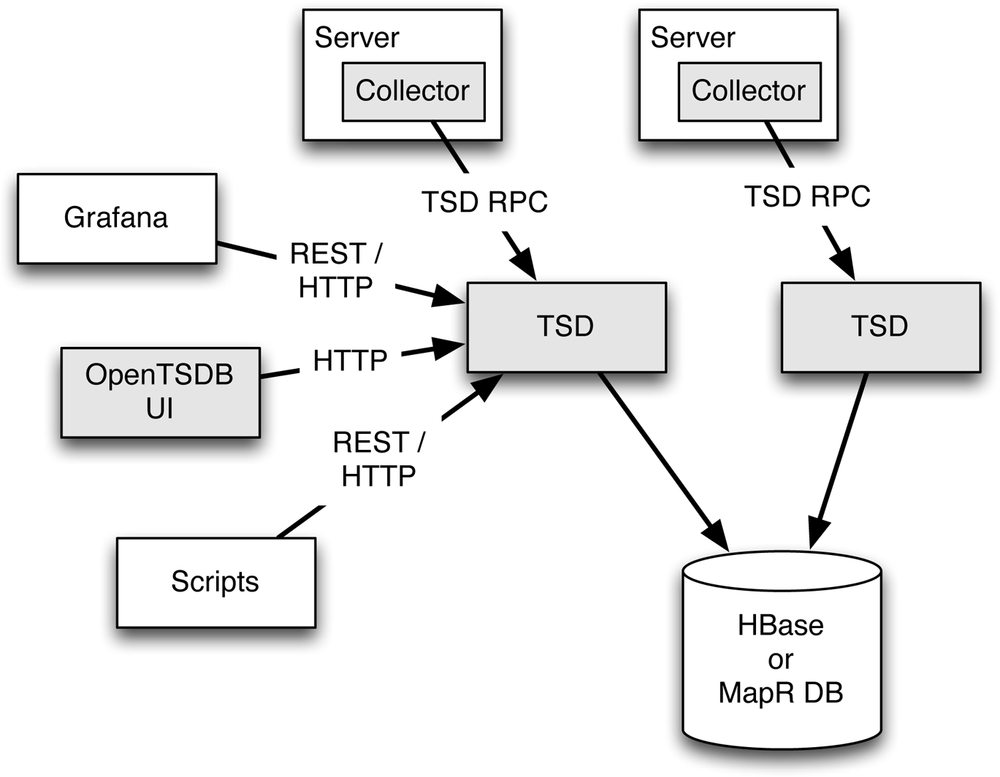
On servers where measurements are made, there is a collector process that sends data to the time series daemon (TSD) using the TSD RPC protocol. The time series daemons are responsible for looking up the time series to which the data is being appended and inserting each data point as it is received into the storage tier. A secondary thread in the TSD later replaces old rows with blob-formatted versions in a process known as row compaction. Because the TSD stores data into the storage tier immediately and doesn’t keep any important state in memory, you can run multiple TSD processes without worrying about them stepping on each other. The TSD architecture shown here corresponds to the data flow depicted in the previous chapter in Figure 3-5 to produce hybrid-style tables. Note that the data catcher and the background blob maker of that figure are contained within the TSD component shown here in Figure 4-1.

User interface components such as the original Open TSDB user interface communicate directly with the TSD to retrieve data. The TSD retrieves the requested data from the storage tier, summarizes and aggregates it as requested, and returns the result. In the native Open TSDB user interface, the data is returned directly to the user’s browser in the form of a PNG plot generated by the Gnuplot program. External interfaces and analysis scripts can use the PNG interface, but they more commonly use the REST interface of Open TSDB to read aggregated data in JSON form and generate their own visualizations.

Open TSDB suffers a bit in terms of ingestion performance by having collectors to send just a few data points at a time (typically just one point at a time) and by inserting data in the wide table format before later reformatting the data into blob format (this is the standard hybrid table data flow). Typically, it is unusual to be able to insert data into the wide table format at higher than about 10,000 data points per second per storage tier node. Getting ingestion rates up to or above a million data points per second therefore requires a large number of nodes in the storage tier. Wanting faster ingestion is not just a matter of better performance always being attractive; many modern situations produce data at such volume and velocity that in order be able to store and analyze it as a time series, it’s necessary to increase the data load rates for the time series database in order to the do the projects at all.

This limitation on bulk ingestion speed can be massively improved by using an alternative ingestion program to directly write data into the storage tier in blob format. We will describe how this works in the next section.

Value Added: Direct Blob Loading for High Performance

An alternative to inserting each data point one by one is to buffer data in memory and insert a blob containing the entire batch. The trick is to move the blob maker upstream of insertion into the storage tier as described in Chapter 3 and Figure 3-6. The first time the data hits the table, it is already compressed as a blob. Inserting entire blobs of data this way will help if the time windows can be sized so that a large number of data points are included in each blob. Grouping data like this improves ingestion performance because the number of rows that need to be written to the storage tier is decreased by a factor equal to the average number of points in each blob. The total number of bytes may also be decreased if you compress the data being inserted. If you can arrange to have 1,000 data points or more per blob, ingest rates can be very high. As mentioned in Chapter 3, in one test with one data point per second and one-hour time windows, ingestion into a 4-node storage tier in a 10-node MapR cluster exceeded 100 million data points per second. This rate is more than 1,000 times faster than the system was able to ingest data without direct blob insertion.

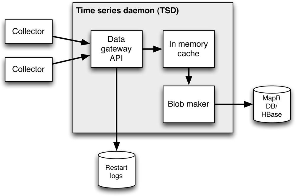
To accomplish this high-performance style of data insertion with live data arriving at high velocity as opposed to historical data, it is necessary to augment the native Open TSDB with capabilities such as those provided by the open source extensions developed by MapR and described in more detail in the following section. Figure 4-2 gives us a look inside the modified time series daemon (TSD) as modified for direct blob insertion. These open source modifications will work on databases built with Apache HBase or with MapR-DB.

Figure 4-2. Changes inside the TSD when using extensions to Open TSDB that enable high-speed ingestion of rapid streaming data. Data is ingested initially to the storage tier in the blob-oriented format that stores many data points per row.

A New Twist: Rapid Loading of Historical Data

Using the extensions to Open TSDB, it is also possible to set up a separate data flow that loads data in blob-style format directly to the storage tier independently of the TSD. The separate blob loader is particularly useful with historical data for which there is no need to access recent data prior to its insertion into the storage tier. This design can be used at the same time as either a native or a modified TSD is in use for other data sources such as streaming data. The use of the separate blob loader for historical data is shown in Figure 4-3.

Figure 4-3. Historical data can be ingested at high speed through direct blob ingenstion by using the blob loader alongside Open TSDB, without needing an in-memory cache. Additional architectural components are shown grayed out here for context.

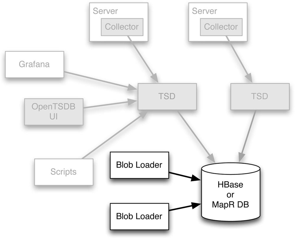
When using this blob loader, no changes are needed to the TSD systems or to the UI components since the blob loader is simply loading data in a format that Open TSDB already uses. In fact, you can be ingesting data in the normal fashion at the same time that you are loading historical data using the blob loader.

The blob loader accelerates data ingestion by short-circuiting the normal load path of Open TSDB. The effect is that data can be loaded at an enormous rate because the number of database operations is decreased by a large factor for data that has a sufficiently large number of samples in each time window.

Since unmodified Open TSDB can only retrieve data from the Apache HBase or MapR-DB storage tier, using the direct bulk loader of the extension means that any data buffered in the blob loader’s memory and not yet written to the data tier cannot be seen by Open TSDB. This is fine for test or historical data, but is often not acceptable for live data ingestion. For test and historical ingestion, it is desirable to have much higher data rates than for production use, so it may be acceptable to use conventional ingestion for current data and use direct bulk only for other testing and backfill.

Summary of Open Source Extensions to Open TSDB for Direct Blob Loading

The performance acceleration available with open source MapR extensions to TSDB can be used in several ways. These general modes of using the extensions include:

Direct bulk loader

The direct bulk loader loads data directly into storage tier in the Open TSDB blob format. This is the highest-performance load path and is suitable for loading historical data while the TSD is loading current data.

File loader

The file loader loads files via the new TSD bulk API. Loading via the bulk API decreases performance somewhat but improves isolation between components since the file loader doesn’t need to know about internal Open TSDB data formats.

TSD API for bulk loading

This bulk load API is an entry point in the REST API exposed by the TSD component of Open TSDB. The bulk load API can be used in any collector instead of the point-by-point insertion API. The advantage of using the bulk API is that if the collector falls behind for any reason, it will be able to load many data points in each call to the API, which will help it catch up.

In-memory buffering for TSD

The bulk load API is supported by in-memory buffering of data in the TSD. As data arrives, it is inserted into a buffer in the TSD. When a time window ends, the TSD will write the contents of the buffers into the storage tier in already blobbed format. Data buffered in memory is combined with data from the storage tier to satisfy any queries that require data from the time period that the buffer covers.

The current primary use of the direct bulk loader is to load large amounts of historical data in a short amount of time. Going forward, the direct bulk loader may be deprecated in favor of the file loader to isolate knowledge of the internal file formats.

The file loader has the advantage that it uses the REST API for bulk loading and therefore, data being loaded by the file loader will be visible by queries as it is loaded.

These enhancements to Open TSDB are available on github. Over time, it is expected that they will be integrated into the upstream Open TSDB project.

Accessing Data with Open TSDB

Open TSDB has a built-in user interface, but it also allows direct access to time series data via a REST interface. In a few cases, the original data is useful, but most applications are better off with some sort of summary of the original data. This summary might have multiple data streams combined into one or it might have samples for a time period aggregated together. Open TSDB allows reduction of data in this fashion by allowing a fixed query structure.

In addition to data access, Open TSDB provides introspection capabilities that allow you to determine all of the time series that have data in the database and several other minor administrative capabilities.

The steps that Open TSDB performs to transform the raw data into the processed data it returns include:

Selection

The time series that you want are selected from others by giving the metric name and some number of tag/value pairs.

Grouping

The selected data can be grouped together. These groups determine the number of time series that are returned in the end. Grouping is optional.

Down-sampling

It is common for the time series data retrieved by a query to have been sampled at a much higher rate than is desired for display. For instance, you might want to display a full year of data that was sampled every second. Display limitations mean that it is impossible to see anything more than about 1–10,000 data points. Open TSDB can downsample the retrieved data to match this limit. This makes plotting much faster as well.

Aggregation

Data for particular time windows are aggregated using any of a number of pre-specified functions such as average, sum, or minimum.

Interpolation

The time scale of the final results regularized at the end by interpolating as desired to particular standard intervals. This also ensures that all the data returned have samples at all of the same points.

Rate conversion

The last step is the optional conversion from counts to rates.

Each of these steps can be controlled via parameters in the URLs of the REST request that you need to send to the time series daemon (TSD) that is part of Open TSDB.

Working on a Higher Level

While you can use the REST interface directly to access data from Open TSDB, there are packages in a variety of languages that hide most of the details. Packages are available in R, Go, and Ruby for accessing data and more languages for pushing data into Open TSDB. A complete list of packages known to the Open TSDB developers can be found in the Open TSDB documentation in Appendix A.

As an example of how easy this can make access to Open TSDB data, here is a snippet of code in R that gets data from a set of metrics and plots them

result <- tsd_get(metric, start, tags=c(site="*"),
downsample="10m-avg")
library(zoo)
z <- with(result, zoo(value, timestamp))
filtered <- rollapply(z, width=7, FUN=median)
plot(merge(z, filtered))

This snippet is taken from the README for the github project. The first line reads the data, grouping by site and downsampling to 10-minute intervals using an arithmetic average. The second line converts to a time series data type and computes a rolling median version of the data. The last line plots the data.

Using a library like this is an excellent way to get the benefits of the simple conceptual interface that Open TSDB provides combined with whatever your favorite language might be.

Using a package like this to access data stored in Open TSDB works relatively well for moderate volumes of data (up to a few hundred thousand data points, say), but it becomes increasingly sluggish as data volumes increase. Downsampling is a good approach to manage this, but downsampling discards information that you may need in your analysis. At some point, you may find that the amount of data that you are trying to retrieve from your database is simply too large either because downloading the data takes too long or because analysis in tools like R or Go becomes too slow.

If and when this happens, you will need to move to a more scalable analysis tool that can process the data in parallel.

Accessing Open TSDB Data Using SQL-on-Hadoop Tools

If you need to analyze large volumes of time series data beyond what works with the REST interface and downsampling, you probably also need to move to parallel execution of your analysis. At this point, it is usually best to access the contents of the Open TSDB data directly via the HBase API rather than depending on the REST interface that the TSD process provides.

You might expect to use SQL or the new SQL-on-Hadoop tools for this type of parallel access and analysis. Unfortunately, the wide table and blob formats that Open TSDB uses in order to get high performance can make it more difficult to access this data using SQL-based tools than you might expect. SQL as a language is not a great choice for actually analyzing time series data. When it comes to simply accessing data from Open TSDB, the usefulness of SQL depends strongly on which tool you select, as elaborated in the following sections. For some tools, the non-relational data formats used in Open TSDB can be difficult to access without substantial code development. In any case, special techniques that vary by tool are required to analyze time series data from Open TSDB. New SQL-on-Hadoop tools are being developed. In the next sections, we compare some of the currently available tools with regard to how well they let you access your time series database and Open TSDB.

Using Apache Spark SQL

Apache Spark SQL has some advantages in working with time series databases. Spark SQL is very different from Apache Hive in that it is embedded in and directly accessible from a full programming language. The first-class presence of Scala in Spark SQL programs makes it much easier to manipulate time series data from Open TSDB.

In particular, with Spark SQL, you can use an RDD (resilient distributed dataset) directly as an input, and that RDD can be populated by any convenient method. That means that you can use a range scan to read a number of rows from the Open TSDB data tier in either HBase or MapR-DB into memory in the form of an RDD. This leaves you with an RDD where the keys are row keys and the values are HBase Result structures. The getFamilyMap method can then be used to get all columns and cell values for that row. These, in turn, can be emitted as tuples that contain metric, timestamp, and value. The flatmap method is useful here because it allows each data row to be transformed into multiple time series samples.

You can then use any SQL query that you like directly on these tuples as stored in the resulting RDD. Because all processing after reading rows from HBase is done in memory and in parallel, the processing speed will likely be dominated by the cost of reading the rows of data from the data tier. Furthermore, in Spark, you aren’t limited by language. If SQL isn’t convenient, you can do any kind of Spark computation just as easily.

A particularly nice feature of using Spark to analyze metric data is that the framework already handles most of what you need to do in a fairly natural way. You need to write code to transform OpenTSDB rows into samples, but this is fairly straightforward compared to actually extending the platform by writing an input format or data storage module from scratch.

Why Not Apache Hive?

Analyzing time series data from OpenTSDB using Hive is much more difficult than it is with Spark. The core of the problem is that the HBase storage engine for Hive requires that data be stored using a very standard, predefined schema. With Open TSDB, the names of the columns actually contain the time portion of the data, and it isn’t possible to write a fully defined schema to describe the tables. Not only are there a large number of possible columns (more than 10¹⁰⁰⁰), but the names of the columns are part of the data. Hive doesn’t like that, so this fact has to be hidden from it.

The assumptions of Hive’s design are baked in at a pretty basic level in the Hive storage engine, particularly with regard to the assumption that each column in the database represents a single column in the result. The only way to have Hive understand OpenTSDB is to clone and rewrite the entire HBase storage engine that is part of Hive. At that point, each row of data from the OpenTSDB table can be returned as an array of tuples containing one element for time and one for value. Each such row can be exploded using a lateral view join.

While it is possible to use Hive to analyze Open TSDB data, it is currently quite difficult. Spark is likely a better option.

Adding Grafana or Metrilyx for Nicer Dashboards

The default user interface for Open TSDB is very basic and not suitable for building embedded dashboards; it definitely is a bit too prickly for most ordinary users. In addition, the plots are produced using a tool called Gnuplot, whose default plot format looks very dated. A more convenient visualization interface is desirable.

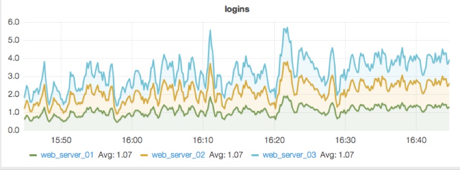
One good solution is the open source dashboard editor known as Grafana. The Open TSDB REST API can provide access to data, and the team behind the Grafana project has used that access to build a high-quality data visualization interface for Open TSDB and other time series databases such as InfluxDB. A sample result is shown in Figure 4-4.

Figure 4-4. A sample plot from Grafana. This plot is taken from the sample instance that can be accessed from the project home page.

Installation of Grafana is quite simple because it runs entirely on the client side using JavaScript. All you need to run Grafana is a web server that can serve static files such as Twistd or nginx. You will also have to make sure that your users’ browsers can access the Open TSDB REST interface either directly or through a proxy. Using a proxy is a good idea if you want to ensure that users see data but can’t modify it. If you want to allow users to define new dashboards, you will need to install and run an Elasticsearch instance as well. Grafana is available at http://grafana.org/.

Another option for nicer dashboards with Open TSDB is Metrilyx, a package recently open sourced by Ticketmaster. Installing Metrilyx is a bit more involved than installing Grafana because there are additional dependencies (on nginx, Elasticsearch, Mongo and, optionally, Postgres), but there are some benefits such as the use of websockets in order to improve the responsiveness of the display. Keep in mind that while Metrilyx has been in use inside Ticketmaster for some time, it has only recently been released as open source. There may be some teething issues as a result due to the change in environment. Metrilyx is available at https://github.com/Ticketmaster/metrilyx-2.0.

Possible Future Extensions to Open TSDB

The bulk API extension to Open TSDB’s REST interface assumes that data can be buffered in memory by the TSD. This violates the design assumptions of Open TSDB by making the TSD keep significant amounts of state information in memory. This has several negative effects, the most notable being that a failure of the TSD will likely cause data loss. Even just restarting a TSD process means that there is a short moment in time when there is no process to handle incoming data.

In the original Open TSDB design, this was never a problem because TSD processes are stateless by design. This means that you can run several such processes simultaneously and simply pick one at random to handle each API request. Each request that delivers data to the TSD will cause an immediate update of the storage tier, and all requests that ask the TSD are satisfied by reference to the database.

With in-memory buffering, the TSD is no longer stateless, and we therefore lose the benefits of that design. These issues do not affect the use of the bulk API for loading historical or test data because we can simply dedicate a TSD for bulk loading, restarting loading if the TSD fails or needs to be restarted. Similarly, the direct bulk loader is not affected by these considerations.

At this time, the in-memory caching that has been implemented in association with the bulk API has no provisions to allow restarts or multiple TSD processes. The next section describes one design that will support these capabilities safely.

Cache Coherency Through Restart Logs

Ultimately, it is likely to be desirable to allow multiple TSDs to be run at the same time and still use the in-memory caching for performance. This however, leads to a situation where new data points and requests for existing data could go to any TSD at all. In order to ensure that all TSDs have consistent views of all data, we need to have a cache coherency protocol where all new data accepted by any TSD has a very high likelihood of being present on every TSD very shortly after it arrives.

In order to do this simply, we require all TSDs to write restart logs that contain a record of all the transactions that they have received as well as a record of exactly when blobs are written to the storage tier. All TSDs can then read the restart logs of all of the other TSDs. This will help in two ways. First, all TSDs, including those recently started, will have very nearly identical memory states. Secondly, only one TSD will actually write each row to the database. Such a design avoids nearly all coordination at the cost of requiring that all recent data points be kept in multiple TSD memory spaces.

This design requires that a TSD be able to read restart logs and modify its in-memory representation at the full production data rate, possibly using several hardware threads. Since restart logs are kept in conventional flat files, reading the data in a binary format at high rates is not a problem. Likewise, since the cache is kept in memory, updating the cache at more than a million updates per second is likewise not a major problem.

The only remaining issue is to arrange for only one TSD to write each row to the database. This can be done by having each TSD pick a random time to wait before writing an idle dirty row back to the database. When the TSD starts the write, it will write a start transaction to the log, and when it completes the write, it will write a finish transaction to the log. When other TSDs read the finish transaction from the first TSD’s restart log, they will silently discard the dirty row if their last update time matches the update time that was written to the database. Any TSD that reads a start transaction will delay its own write time for that row by a few seconds to allow the finish operation to arrive. By setting the range of the random times large with respect to the time required to propagate the start transaction, the probability that two TSDs will start a write on the same row can be made very, very small. Even if two TSDs do decide to write the same row to the database, row updates are atomic, so the two processes will write the same data (since the row is idle at this point). The net effect is that each row will almost always be written to the database only once, on average.

With an understanding of basic concepts related to building a large scale, NoSQL time series database provided by Chapter 3 and the exploration of open source tools to implement those ideas, as described here in Chapter 4, you should now be well prepared to tackle your own project with time series data. But before you do, consider how one of the options described here can fix a problem you might not yet know exists. Chapter 5 shows you how.