Understanding the tools of the performance analyst’s trade is essential for approaching matters of Windows 2000 performance. Rather than focus merely on tools and how they work, we chose to emphasize the use of analytic techniques to diagnose and solve performance problems. We stress an empirical approach, making observations of real systems under stress. If you are a newcomer to the Microsoft operating system but understand how Unix, Linux, Solaris, OpenVMS, MVS, or another full-featured OS works, you will find much that is familiar here. Moreover, despite breathtaking changes in computer architecture, many of the methods and techniques used to solve earlier performance problems can still be applied successfully today. This is a comforting thought as we survey the complex computing environments, a jumbled mass of hardware and software alternatives, that we are called upon to assess, configure, and manage today. Measurement methodology, workload characterization, benchmarking, decomposition techniques, and analytic queuing models remain as effective today as they were for the pioneering individuals who first applied these methods to problems in computer performance analysis.
Computer performance evaluation is significant because it is very closely associated with the productivity of the human users of computerized systems. Efficiency is the principal rationale for computer-based automation. Whenever productivity is a central factor in decisions regarding the application of computer technology to automate complex and repetitive processes, performance considerations loom large. These concerns were present at the dawn of computing and remain very important today. Even as computing technology improves at an unprecedented rate, the fact that our expectations of this technology grow at an even faster rate assures that performance considerations will continue to be important in the future.
In computer performance, productivity is often tangled up with cost. Unfortunately, the relationship between performance and cost is usually neither simple nor straightforward. Generally, more expensive equipment has better performance, but there are many exceptions. Frequently, equipment will perform well with some workloads but not others. In most buying decisions, it is important to understand the performance characteristics of the hardware, the performance characteristics of the specific workload, and how they match up with each other.
In a sea of change, computer performance is one of the few areas of computing to remain relatively constant. As computing paradigms shift, specific areas of concern to performance analysts are subject to adjustment and realignment. Historically, the central server model of mainframe computing was the focus of much performance analysis in the 1960s and early 1970s. Understanding the performance of timesharing systems with virtual memory motivated basic research. Today, the focus has shifted to the performance of client/server applications, two- and three-tiered architectures, web-enabled transaction processing applications, internetworking, electronic mail and other groupware applications, databases, and distributed computing. Windows 2000 is at the center of many of these trends in desktop, networking, and enterprise computing, which is why Windows 2000 performance remains a critical concern.
To be able to evaluate the performance of a computer system, you need a thorough understanding of the important metrics used to measure computer performance. Computers are machines designed to perform work, and we measure their capacity to perform the work, the rate at which they are currently performing it, and the time it takes to perform specific tasks. In the following sections, we look at some of the key ways to measure computer performance, introducing the most commonly used metrics: bandwidth, throughput, service time, utilization, and response time.
Bandwidth measures the capacity of a link, bus, channel, interface, or device to transfer data. It is usually measured in either bits/second or bytes/second (there are eight bits in a data byte). For example, the bandwidth of a 10BaseT Ethernet connection is 10 Mb/sec, the bandwidth of a SCSI-2 disk is 20 MB/sec, and the bandwidth of the PCI Version 2.1 64-bit 66 MHz bus is 528 MB/sec.
Bandwidth usually refers to the maximum theoretical data transfer
rate of a device under ideal conditions, and, therefore, it needs to
be treated as an upper bound of performance. You
can rarely measure the device actually performing at that rate, as
there are many reasons why the theoretical bandwidth is not
achievable in real life. For instance, when an application transfers
a block of information to the disk, various layers of the operating
system (OS) normally need to process the request first. Also, before
a requested block of data can be transferred across a channel to the
disk, some sort of handshaking protocol is required to set up the
hardware operation. Finally, at the physical disk itself, your
request is likely to be delayed during the time it takes to position
the read/write actuator of the disk over the designated section on
the rotating magnetic platter. The unavoidable
overhead of operating system software, protocol
message exchange, and disk positioning absorbs some of the available
bandwidth so the application cannot use the full rated bandwidth of
the disk for data transfer.
To provide another example, in networking people are accustomed to speaking about the bandwidth of a LAN connection to transfer data in millions of bits per second. Consider an application that seeks to transfer an IP packet using the UDP protocol on an Ethernet network. The actual packet, when it reaches your network hardware, looks like Figure 1-1, with additional routing and control information added to the front of the message by various networking software layers.
The datagram illustrated in Figure 1-1 is then passed to a network interface card (NIC) attached to the LAN. As the NIC generates the bit stream that it places on the LAN connection wire, it adds two error check bits for every eight data bits in the original payload. This 10/8 bit encoding scheme implemented at the Ethernet physical link layer reduces the effective bandwidth of the network connection proportionally. Assuming that nobody else is using the network when the packet arrives at the Ethernet interface, and that the full bandwidth is used for the transfer of this packet, we can calculate the actual bandwidth observed by the user for this particular data transfer using the following expression:

or:
The maximum effective bandwidth that can be observed by the user in
this case is 7.34 Mb/sec. If there is congestion on the network,
leading to collisions on an Ethernet network,
the actual observed bandwidth might be substantially lower. As we
will discuss in detail in Chapter 12, it is not
unusual to expect the effective bandwidth of an Ethernet 10 Mb LAN to
be less than 5 Mb/sec.
Throughput
measures the rate at which some sort
of work is actually being done by the system; that is, the rate at
which work is completed as observed by some application. Examples of
throughput measurements include the number of reads per second from
the filesystem, the number of instructions per second executed by the
processor, the number of HTTP requests processed by a web server, and
the number of transactions per second that can be processed by a
database engine.
Throughput and bandwidth are very
similar. Bandwidth is often construed as the capacity
of the system to perform work, while throughput is the
current observed rate at which that work is being performed.
Understanding that the throughput of a particular system is starting
to approach its effective capacity limits is something very important
to know. It means, for example, that no amount of tweaking of
esoteric tuning parameters is going to overcome the capacity
constraint and allow the system to perform more work. The only
effective solution that will allow you to perform more work is to
upgrade the component of the system that is functioning at or near
its effective bandwidth limits. Alternatively, you may be able to
tune the application so that it runs more efficiently (i.e., utilizes
less bandwidth) against the specific resource, or split the
application somehow across multiple processing engines (processors,
disks, network segments, etc.).
Service time
measures how long it takes to process a
specific request. Engineers also often speak of the length of time
processing a request as the device’s
latency, another word for delay. Other related
measures of service time are the turnaround time
for requests, usually ascribed to longer running tasks, such as
disk-to-tape backup runs, and the round trip
time, an important measure of network latency because when
a request is sent to a destination, the sender must wait for a reply.
There is no substitute for direct measurements of device or application service time. The service time of a filesystem request, for example, will vary based on whether the request is cached in memory or requires a physical disk operation. The service time will also vary depending on if it’s a sequential read, a random read, or a write. The expected service time of the physical disk request also varies depending on the block size of the request. These workload dependencies demand that you measure disk service time directly, instead of relying on some idealized model of disk performance expectations.
The
service time spent processing a web application request can be broken
down into processing components: for example, time spent in the
application script, time spent in the operating system, and time
spent in database processing. For each one of these subcomponents, we
might further decompose the application service time into time spent
at various hardware components, the CPU, the disk, the network, etc.
Decomposition is one of the fundamental
techniques used in computer performance analysis to relate a workload
to its various hardware and software processing components. To allow
us to decompose application service times into their component parts,
we must understand how busy various hardware components are and how
specific workloads contribute to that utilization.
Utilization
measures the fraction of time that a
device is busy servicing requests, usually reported as a percent
busy. Utilization of a device varies between 0 and 1, where 0 is idle
and 1 represents utilization of the full bandwidth of the device. It
is customary to report that the CPU is 75% busy or the disk is 40%
busy. It is not possible for a single device to ever appear more than
100% busy.
The utilization of a device is related directly to the observed throughput (or request rate) and service time as follows:
| Utilization = Throughput x Service Time |
This simple formula relating device utilization, throughput, and service time is known as the Utilization Law. The Utilization Law makes it possible to measure the throughput and service time of a disk, for example, and derive the disk utilization. For example, a disk that processes 20 input/output (I/O) operations per second with an average service time of 10 milliseconds is busy processing requests 20 x 0.010 every second, and is said to be 20% busy.
Alternatively, we might measure the utilization of a device using a sampling technique while also keeping track of throughput. Using the Utilization Law, we can then derive the service time of requests. Suppose we sample a communications bus 1000 times per second and find that it is busy during 200 of those measurements, or 20%. If we measure the number of bus requests at 2000 per second over the same sampling interval, we can derive the average service time of bus requests equal to 0.2 ÷ 2000 = .0001 seconds or 100 microseconds (μsecs).
Monitoring the utilization of various hardware components is an important element of capacity planning. Measuring utilization is very useful in detecting system bottlenecks, which are essentially processing constraints due to limits on the effective throughput capacity of some overloaded device. If an application server is currently processing 60 transactions per second with a CPU utilization measured at 20%, the server apparently has considerable reserve capacity to process transactions at an even higher rate. On the other hand, a server processing 60 transactions per second running at a CPU utilization of 98% is operating at or near its maximum capacity.
Unfortunately, computer capacity planning
is not as easy as projecting that the server running at 20% busy
processing 60 transactions per second is capable of processing 300
transactions per second. You would not need to read a big, fat book
like this one if that were all it took. Because transactions use
other resources besides the CPU, one of those other resources might
reach its effective capacity limits long before the CPU becomes
saturated. We designate the component functioning as the constraining
factor on throughput as the bottlenecked device.
Unfortunately, it is not always easy to identify the bottlenecked
device in a complex, interrelated computer system or network of
computer systems.
It
is safe to assume that devices observed operating at or near their
100% utilization limits are bottlenecks, although things are not
always that simple. For one thing, 100% is not necessarily the target
threshold for all devices. The effective capacity of an Ethernet
network normally decreases when the utilization of the network
exceeds 40-50%. Ethernet LANs use a shared link, and packets intended
for different stations on the LAN can collide
with one another, causing delays. Because of the way Ethernet works,
once line utilization exceeds 40-50%, collisions start to erode the
effective capacity of the link. We will talk about this phenomenon in
much more detail in Chapter 11.
As the utilization of shared components increases, processing delays are encountered more frequently. When the network is heavily utilized and Ethernet collisions occur, for example, NICs are forced to retransmit packets. As a result, the service time of individual network requests increases. The fact that increasing the rate of requests often leads to processing delays at busy shared components is crucial. It means that as we increase the load on our server from 60 transactions per second and bottlenecks in the configuration start to appear, the overall response time associated with processing requests will not hold steady. Not only will the response time for requests increase as utilization increases, it is likely that response time will increase in a nonlinear relationship to utilization. In other words, as the utilization of a device increases slightly from 80% to 90% busy, we might observe that the response time of requests doubles, for example.
Response
time
, then, encompasses both the service time
at the device processing the request and any other delays encountered
waiting for processing. Formally, response time is defined as:
| Response time = service time + queue time |
where queue time represents the amount of time a request waits for service. In general, at low levels of utilization, there is minimal queuing, which allows device service time to dictate response time. As utilization increases, however, queue time increases nonlinearly and, soon, begins to dominate response time.
Queues are essentially data structures where requests for service are parked until they can be serviced. Examples of queues abound in Windows 2000, and measures showing the queue length or the amount of time requests wait in the queue for processing are some of the most important indicators of performance bottlenecks discussed here. The Windows 2000 queues that will be discussed in this book include the operating system’s thread scheduling queue, the logical and physical disk queues, the file server request queue, and the queue of Active Server Pages (ASP) web server script requests. Using a simple equation known as Little’s Law, which is discussed later, we will also show how the rate of requests, the response time, and the queue length are related. This relationship, for example, allows us to calculate average response times for ASP requests even though Windows 2000 does not measure the response time of this application directly.
In performance monitoring, we try to identify devices with high utilizations that lead to long queues where requests are delayed. These devices are bottlenecks throttling system performance. Intuitively, what can be done about bottlenecks once you have discovered one? Several forms of medicine can be prescribed:
Upgrade to a faster device
Spread the workload across multiple devices
Reduce the load on the device by tuning the application
Change scheduling parameters to favor cherished workloads
These are hardly mutually exclusive alternatives. Depending on the situation, you may wish to try more than one of them. Common sense dictates which alternative you should try first. Which change will have the greatest impact on performance? Which configuration change is the least disruptive? Which is the easiest to implement? Which is possible to back out of in case it makes matters worse? Which involves the least additional cost? Sometimes, the choices are fairly obvious, but often these are not easy questions to answer.
One complication is that there
is no simple relationship between response time and device
utilization. In most cases it is safe to assume the underlying
relationship is nonlinear. A peer-to-peer Ethernet LAN experiencing
collisions, for example, leads to sharp increases in both network
latency and utilization. A Windows 2000 multiprocessor implementing
priority queuing with preemptive scheduling at the processor leads to
a categorically different relationship between response time and
utilization, where low-priority threads are subject to a condition
called starvation. A SCSI disk that supports
tagged command queuing can yield higher throughput with lower service
times at higher request rates. In later
chapters, we explore in much more detail the performance
characteristics of the scheduling algorithms that these hardware
devices use, each of which leads to a fundamentally different
relationship between utilization and response time.
This nonlinear relationship between utilization and response time often serves as the effective capacity constraint on system performance. Just as customers encountering long lines at a fast food restaurant are tempted to visit the fast food chain across the way when delays are palpable, customers using an Internet connection to access their bank accounts might be tempted to switch to a different financial institution if it takes too long to process their requests. Consequently, understanding the relationship between response time and utilization is one of the most critical areas of computer performance evaluation. It is a topic we will return to again and again in the course of this book.
Response time measurements are also important for another reason. For example, the response time for a web server is the amount of time it takes from the instant that a client selects a hyperlink to the time that the requested page is returned and displayed on her display monitor. Because it reflects the user’s perspective, the overall response time is the performance measure of greatest interest to the users of a computer system. It is axiomatic that long delays cause user dissatisfaction with the computer systems they are using, although this is usually not a straightforward relationship either. Human factors research, for instance, indicates that users may be more bothered by unexpected delays than by consistently long response times that they have become resigned to.
Intuitively, it may seem that proper configuration and tuning of any computer system or network should attempt to maximize throughput and minimize response time simultaneously. In practice, that is often not possible. For example, system administrators that try to optimize throughput are apt to drive up response time to unacceptable levels as a result. Alternatively, minimizing response time by stockpiling only the fastest and most expensive equipment and then keeping utilization low in order to minimize queuing delays is not very cost-effective. In practice, skilled performance analysts attempt to achieve a balance between these often conflicting objectives:
There is relatively high throughput leading to the cost-effective use of the hardware.
Queuing delays are minimal, so users are satisfied with performance levels.
System performance is relatively stable, consistent, and predictable.
To explain that these objectives are not so easy to reconcile, it may help to take an introductory look at queuing theory, a branch of operations research frequently applied to the analysis of computer systems performance.
Figure 1-2 shows the conventional representation of a queuing system, with customer requests arriving at a server with a simple queue. These are the basic elements of a queuing system: customers, servers, and a queue. Figure 1-2 shows a single server, but multiple-server models are certainly possible.
If the server is idle, customer
requests arriving at the server are processed immediately. On the
other hand, if the server is already busy, then the request is
queued. If multiple requests are waiting in the server queue, the
queuing
discipline
determines the order in which queued requests
are serviced. The simplest and fairest way to order the queue is to
service requests in the order in which they arrive. This is also
called FIFO (First In, First Out) or sometimes First Come, First
Served (FCFS). There are many other ways that a queue of requests can
be ordered, including by priority or by the speed with which they can
be processed.
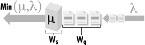
Figure 1-3 shows a simple queue annotated with
symbols that represent a few of the more common parameters that
define its behavior. There are a large number of parameters that can
be used to describe the behavior of this simple queue, and we only
look at a couple of the more basic and commonly used ones.
Response time (W) represents the total amount of
time a customer request spends in the queuing system, including both
service time (Ws) at the
device and wait time (Wq)
in the queue. By convention, the Greek letter λ (lambda) is used
to specify the arrival rate or frequency of
requests to the server. Think of the arrival rate as an activity rate
such as the rate at which HTTP GET requests arrive at a web server,
I/O requests are sent to a disk, or packets are sent to a NIC card.
Larger values of λ indicate that a more intense workload is
applied to the system, whereas smaller values indicate a light load.
Another Greek letter, μ, is used to represent the rate at which
the server can process requests. The output from the server is either
λ or μ, whichever is less, because it is certainly possible
for requests to arrive at a server faster than they can processed.
Ideally, we hope that the arrival
rate is lower than the service rate of the server, so that the server
can keep up with the rate of customer requests. In that case, the
arrival rate is equal to the completion rate, an important
equilibrium assumption that allows us to consider models that are
mathematically tractable (i.e., solvable). If the arrival rate λ
is greater than the server capacity μ, then requests begin
backing up in the queue. Mathematically, arrivals are drawn from an
infinite population so that when λ > μ, the queue length
and the wait time
(Wq
) at the server
grow infinitely large. Those of us who have tried to retrieve a
service pack from a Microsoft web server immediately after its
release know this situation and its impact on performance.
Unfortunately, it is not possible to solve a queuing model with
λ > μ, although mathematicians have developed
heavy traffic approximations to deal with this
familiar case.
In real-world situations, there are limits on the population of customers. The population of customers in most realistic scenarios involving computer or network performance is limited by the number of stations on a LAN, the number of file server connections, the number of TCP connections a web server can support, or the number of concurrent open files on a disk. Even in the worst bottlenecked situation, the queue depth can only grow to some predetermined limit. When enough customer requests are bogged down in queuing delays, in real systems, the arrival rate for new customer requests becomes constrained. Customer requests that are backed up in the system choke off the rate at which new requests are generated.
The
purpose of this rather technical discussion is twofold. First, it is
necessary to make an unrealistic assumption about arrivals being
drawn from an infinite population to generate readily solvable
models. Queuing models break down when λ
→ μ, which is
another way of saying they break down near 100% utilization of some
server component. Second, you should not confuse a queuing model
result that shows a nearly infinite queue length with reality. In
real systems there are practical limits on queue depth. In the
remainder of our discussion here, we will assume that λ <
μ. Whenever the arrival rate of customer requests is equal to the
completion rate, this can be viewed as an
equilibrium
assumption.
Please keep in mind that the following results are invalid if the
equilibrium assumption does not hold; in other words, if the arrival
rate of requests is greater than the completion rate (λ >
μ over some measurement interval) simple queuing models do not
work.
A fundamental result in queuing theory known as Little’s Law relates response time and utilization. In its simplest form, Little’s Law expresses an equivalence relation between response time W, arrival rate λ, and the number of customer requests in the system Q (also known as the queue length):
| Q = λx W |
Note that in this context the queue length Q refers both to customer requests in service (Qs) and waiting in a queue (Qq) for processing. In later chapters we will have several opportunities to take advantage of Little’s Law to estimate response time of applications where only the arrival rate and queue length are known. Just for the record, Little’s Law is a very general result that applies to a large class of queuing models. While it does allow us to estimate response time in a situation where we can measure the arrival rate and the queue length, Little’s Law itself provides no insight into how response time is broken down into service time and queue time delays.
Little’s Law is an important enough result that it is probably worth showing how to derive it. As mentioned, Little’s Law is a very general result in queuing theory—only the equilibrium assumption is required to prove it. Figure 1-4 shows some measurements that were made at disk at discrete intervals shown on the X axis. The Y axis indicates the number of disk requests during the interval. Our observation of the disk is delimited by the two arrows between the start time and the stop time. When we started monitoring the disk, it was idle. Then, whenever an arrival occurred at a certain time, we incremented the arrivals counter. That variable is plotted using the thick line. Whenever a request completed service at the disk, we incremented the completions variable. The completions are plotted using the thin line.
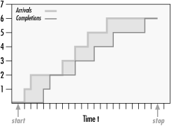
The difference between the arrival and completion lines is the number of requests at the disk at that moment in time. For example, at the third tick-mark on the X axis to the right of the start arrow, there are two requests at the disk, since the arrival line is at 2 and the completion line is at 0. When the two lines coincide, it means that the system is idle at the time, since the number of arrivals is equal to the number of departures.
To calculate the average number of requests in the system during our measurement interval, we need to sum the area of the rectangles formed by the arrival and completion lines and divide by the measurement interval. Let’s define the more intuitive term “accumulated time in the system” for the sum of the area of rectangles between the arrival and completion lines, and denote it by the variable P. Then we can express the average number of requests at the disk, N, using the expression:
We can also calculate the average response time, R, that a request spends in the system (Ws + Wq) by the following expression:
where C is the completion rate (and C = λ, from the equilibrium assumption). This merely says that the overall time that requests spent at the disk (including queue time) was P, and during that time there were C completions. So, on average, each request spent P/C units of time in the system.
Now, all we need to do is combine these two equations to get the magical Little’s Law:
Little’s Law says that the average number of requests in the system is equal to the product of the rate at which the system is processing the requests (with C = λ, from the equilibrium assumption) times the average amount of time that a request spends in the system.
To make sure that this new and important law makes sense, let’s apply it to our disk example. Suppose we collected some measurements on our system and found that it can process 200 read requests per second. The Windows 2000 System Monitor also told us that the average response time per request was 20 ms (milliseconds) or 0.02 seconds. If we apply Little’s Law, it tells us that the average number of requests at the disk, either in the queue or actually in processing, is 200 x 0.02, which equals 4. This is how Windows 2000 derives the Physical Disk Avg. Disk Queue Length and Logical Disk Avg. Disk Queue Length counters. More on that topic in Chapter 8.
Tip
The explanation and derivation we have provided for Little’s Law is very intuitive and easy to understand, but it is not 100% accurate. A more formal and mathematically correct proof is beyond the scope of this book. We followed the development of Little’s Law and notation used by a classic book on queuing networks by Lazowska, Zahorjan, Graham, and Sevcik called Quantitative System Performance: Computer System Analysis Using Queuing Network Models. This is a very readable book that we highly recommend if you have any interest in analytic modeling. Regardless of your interest in mathematical accuracy, though, you should become familiar with Little’s Law. There are occasions in this book where we use Little’s Law to either verify or improve upon some of the counters that are made available in Windows 2000 through the System Monitor. Even if you forget everything else we say here about analytic modeling, don’t forget the formula for Little’s Law.
For a simple class of queuing models, the mathematics to solve them is also quite simple. A simple case is where the arrival rate and service time are randomly distributed around the average value. The standard notation for this class of model is M/M/1 (for the single-server case) and M/M/n (for multiple servers). M/M/1 models are useful because they are easy to compute—not necessarily because they model reality precisely. We can derive response time for an M/M/1 or M/M/n model with FIFO queuing if the arrival rate and service time are known using the following simple formula:
where u is the utilization
of the server, Wq is the queue time,
Ws is the service time, and
Wq
+
Ws = W. As long as we remember that this model
breaks down as utilization approaches 100%, we can use it with a fair
degree of confidence.
Figure 1-5 shows a typical application of this formula for Ws = 10 ms, demonstrating that the relationship between the queue time Wq and utilization is nonlinear. Up to a point, queue time increases gradually as utilization increases, and then each small incremental increase in utilization causes a sharp increase in response time. Notice that there is an inflection point or “knee” in the curve where this nonlinear relationship becomes marked. (If you want an empirical description of the knee in the curve, find the inflection point on the curve where the slope = 1.) Notice also that as the utilization u → 1, the denominator term 1 - u → 0 where Wq is undefined. This accounts for the steep rise in the right-hand portion of the curve as u → 1.
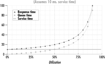
The graph in Figure 1-5 illustrates the various reasons why it is so hard to optimize for both maximum throughput and minimal queue time delays:
As we push a computer system toward its maximum possible throughput, we also force response time to increase rapidly.
Reaching for maximum throughput also jeopardizes stability. Near the maximum throughput levels, slight fluctuations in the workload cause disproportionately large changes in the amount of queue time delay that transactions experience.
Maintaining the stability of application response time requires low utilization levels, which may not be cost-effective.
Figure 1-5 strongly suggests that the three objectives we set earlier for performance tuning and optimization are not easily reconcilable, which certainly makes for interesting work. Having an impossible job to perform at least provides for built-in job security.
For the sake of a concrete example, let us return to our example of the wait queue for a disk. As in Figure 1-5, let’s assume that the average service time Ws at the disk is 10 ms. When requests arrive and the disk is free, requests can be processed at a maximum rate of 1/Ws (1 ÷ 0.010) or 100 requests per second. That is the capacity of the disk. Τ ο maximize throughput, we should keep the disk constantly busy so that it can reach its maximum capacity and achieve throughput of 100 requests/sec. But to minimize response time, the queue should always be kept empty so that the total amount of time it takes to service a request is as close to 10 milliseconds as possible.
If we could control the arrival of customer requests (perhaps through scheduling) and could time each request so that one arrived every Ws seconds (once every 10 ms), we would improve performance. When requests are paced to arrive regularly every 10 milliseconds, the disk queue is always empty and the request can be processed immediately. This succeeds in making the disk 100% busy, attaining its maximum potential throughput of 1/Ws requests per second. With perfect scheduling and perfectly uniform service times for requests, we can achieve 100% utilization of the disk with no queue time delays.
In reality, we have little
or no control over when I/O requests arrive at the disk in a typical
computer system. In a typical system, there are periods when the
server is idle and others when requests arrive in bunches. Moreover,
some requests are for large amounts of data located in a distant spot
on the disk, while others are for small amounts of data located near
the current disk actuator. In the language of queuing theory, neither
the arrival rate distribution of customer
requests or the service time distribution is
uniform. This lack of uniformity causes some requests to queue, with
the further result that as the throughput starts to approach the
maximum possible level, significant queuing delays occur. As the
utilization of the server increases, the response time for customer
requests increases significantly during periods of congestion, as
illustrated by the behavior of the simple M/M/1 queuing model in
Figure 1-5.
[1]
This brief mathematical foray is intended to illustrate the idea that attempting to optimize throughput while at the same time minimizing response is inherently difficult, if not downright impossible. It also suggests that any tuning effort that makes the arrival rate or service time of customer requests more uniform is liable to be productive. It is no coincidence that this happens to be the goal of many popular optimization techniques. It further suggests that a good approach to computer performance tuning and optimization should stress analysis, rather than simply dispensing advice about what tuning adjustments to make when problems occur.
We believe that the first thing you should do whenever you encounter a performance problem is to measure the system experiencing the problem and try to understand what is going on. Computer performance evaluation begins with systematic empirical observations of the systems at hand.
In seeking to understand the root cause of many performance problems, we rely on a mathematical approach to the analysis of computer systems performance that draws heavily on insights garnered from queuing theory. Ever notice how construction blocking one lane of a three-lane highway causes severe traffic congestion during rush hour? We may notice a similar phenomenon on the computer systems we are responsible for when a single component becomes bottlenecked and delays at this component cascade into a problem of major proportions. Network performance analysts use the descriptive term storm to characterize the chain reaction that sometimes results when a tiny aberration becomes a bigproblem. Long before chaos theory, it was found that queuing models of computer performance can accurately depict this sort of behavior mathematically. Little’s Law predicts that as utilization of a resource increases linearly, response time increases exponentially. This fundamental nonlinear relationship that was illustrated in Figure 1-5 means that quite small changes in the workload can result in extreme changes in performance indicators, especially as important resources start to become bottlenecks.
This is exactly the sort of behavior you can expect to see in the computer systems you are responsible for. Most computer systems do not degrade gradually. Queuing theory is a useful tool in computer performance evaluation because it is a branch of mathematics that models systems performance realistically. The painful reality we face is that performance of the systems we are responsible for is acceptable day after day, until quite suddenly it goes to hell in a handbasket. This abrupt change in operating conditions often begets an atmosphere of crisis. The typical knee-jerk reaction is to scramble to identify the thing that changedand precipitated the emergency. Sometimes it is possible to identify what caused the performance degradation, but more often it is not so simple.
With insights from queuing theory, we learn that it may not be a major change in circumstances that causes a major disruption in current performance levels. In fact, the change can be quite small and gradual and still produce a dramatic result. This is an important perspective to have the next time you are called upon to diagnose a Windows 2000 performance problem. Perhaps the only thing that changed is that a component on the system has reached a high enough level of utilization where slight variations in the workload provoke drastic changes in behavior.
A full exposition of queuing theory and its applications to computer performance evaluation is well beyond the scope of this book. Readers interested in pursuing the subject might want to look at Daniel Mensace’s Capacity Planning and Performance Modeling: From Mainframes to Client/Server Systems; Raj Jain’s encyclopedic The Art of Computer Systems Performance Analysis: Techniques for Experimental Design, Measurement, Simulation, and Modeling; or Arnold Allen’s very readable textbook on Probability, Statistics, and Queuing Theory With Computer Science Applications.
Performance tuning presupposes some form of computer measurement. Understanding what is measured, how measurements are gathered, and how to interpret them is another crucial area of computer performance evaluation. You cannot manage what you cannot measure, but fortunately, measurement is pervasive. Many hardware and software components support measurement interfaces. In fact, because of the quantity of computer measurement data that is available, it is often necessary to subject computer usage to some form of statistical analysis. This certainly holds true on Windows 2000, which can provide large amounts of measurement data. Sifting through all these measurements demands an understanding of a statistical approach known as exploratory data analysis, rather than the more familiar brand of statistics that uses probability theory to test the likelihood that a hypothesis is true or false. John Tukey’s classic textbook entitled Exploratory Data Analysis (currently out of print) or Understanding Robust and Exploratory Data Analysis by Hoaglin, Mosteller, and Tukey provides a very insightful introduction to using statistics in this fashion.
Many of the case studies described in this book apply the techniques of exploratory data analysis to understanding Windows 2000 computer performance. Rather than explore the copious performance data available on a typical Windows 2000 platform at random, however, our search is informed by the workings of computer hardware and operating systems in general, and of Windows 2000, Intel processor hardware, SCSI disks, and network interfaces in particular.
Because graphical displays of information are so important to this process, aspects of what is known as scientific visualization are also relevant. (It is always gratifying when there is an important-sounding name for what you are doing!) Edward Tufte’s absorbing books on scientific visualization, including Visual Explanations and The Visual Display of Quantitative Information, are an inspiration.[2] In many place in this book, we will illustrate the discussion with exploratory data analysis techniques. In particular, we will look for key relationships between important measurement variables. Those illustrations rely heavily on visual explanations of charts and graphs to explore key correlations and associations. It is a technique we recommend highly.
In computer performance analysis, measurements, models, and statistics remain the tools of the trade. Knowing what measurements exist, how they are taken, and how they should be interpreted is a critical element of the analysis of computer systems performance. We will address that topic in detail in Chapter 2, so that you can gain a firm grasp of the measurement data available in Windows 2000, how it is obtained, and how it can be interpreted.
[1] The simple M/M/1 model we discuss here was chosen because it is simple, not because it is necessarily representative of real behavior on live computer systems. There are many other kinds of queuing models that reflect arrival rate and service time distributions different from the simple M/M/1 assumptions. However, although M/M/1 may not be realistic, it is easy to calculate. This contrasts with G/G/1, which uses a general arrival rate and service time distribution, i.e., any kind of statistical distribution: bimodal, symptomatic, etc. No general solution to a G/G/1 model is feasible, so computer modelers are often willing to compromise reality for solvability.
[2] It is no surprise that Professor Tufte is extending Tukey’s legacy of the exploratory data analysis approach, as Tukey is a formative influence on his work.
Get Windows 2000 Performance Guide now with the O’Reilly learning platform.
O’Reilly members experience books, live events, courses curated by job role, and more from O’Reilly and nearly 200 top publishers.

