Chapter 2. The PHY
There’s fifty-seven channels and no free airtime...
Large improvements in 802.11 speeds typically have resulted from the introduction of a big new idea. Introducing multi-carrier transmission with OFDM increased speeds in the transition from 802.11b to 802.11a/g. Creating MIMO systems did the same in the move from 802.11a/g to 802.11n. 802.11ac, however, does not introduce a new way of transmitting data over the air. Though they are both extended beyond what was introduced in 802.11n, the techniques used to put bits on the air in 802.11ac will be familiar to anybody familiar with 802.11n: MIMO and wide channels. Raw speed increases in the PHY come from three sources: a higher number of MIMO streams, wider channels, and a finer modulation that can pack more bits into each unit of airtime.
Extended MIMO Operations
One of the major techniques used by 802.11ac to increase throughput is the extension of MIMO from a system that supports four spatial streams to one that supports eight. As with all other MIMO systems, each spatial stream requires its own transmission system; building an 802.11ac AP that supports eight spatial streams would therefore require an antenna array with eight independent radio chains and antennas. Taken as a single protocol feature, extending to eight spatial streams alone doubles throughput over an equivalent 802.11n system by doing something equivalent to doubling the number of lanes on a highway. It will, however, take time to bring devices with more than four spatial streams to market. Just as in previous versions of 802.11 MIMO systems, a transmitter must have at least one radio chain for transmission for each spatial stream; as devices support more spatial streams, the required antenna has more elements and will grow in size.
Note
The number of spatial streams can be no greater than the number of elements in the antenna array. When the count of array elements exceeds the number of spatial streams, there is an additional signal processing gain that can be used to improve the signal-to-noise ratio in beamforming.
Beamforming is a capability that was first proposed in 802.11n, though it never achieved widespread implementation. By using the antenna array to send carefully phase-shifted energy patterns, it is possible to “steer” a data stream toward a particular receiver. 802.11ac builds on beamforming by allowing multiple simultaneous transmissions for multi-user MIMO (MU-MIMO). MU-MIMO is one of the key technologies that will take 802.11ac far beyond its published (or “headline”) data rate for frame transmission. Instead of having a single transmitter and receiver in the same area, MU-MIMO enables spatial reuse, where the same channel can be used in different areas by the same access point. This exciting development will bring the benefits of switching and reduced collision domains to 802.11 networks. It is a topic that requires its own in-depth exposition because it requires communication between protocol layers; it is discussed fully in Chapter 4.[9]
Radio Channels in 802.11ac
To the well-established 20 MHz channel that has been widely used in 802.11 from the first standardization of OFDM in 802.11a and the 40 MHz channel used in 802.11n, the 802.11ac brings two new channel sizes. As expected, wider channels bring higher throughput. Just as in previous OFDM-based transmission, 802.11ac divides the channel into OFDM subcarriers, each of which has a bandwidth of 312.5 kHz. Each of the subcarriers is used as an independent transmission, and OFDM distributes the incoming data bits among the subcarriers. A few subcarriers are reserved and are called pilot carriers; they do not carry user data and instead are used to measure the channel.
Radio Channel Layout
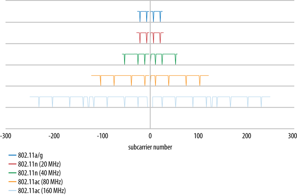
To increase throughput, 802.11ac introduces two new channel widths. All 802.11ac devices are required to support 80 MHz channels, which doubles the size of the spectral channel over 802.11n. It further adds a 160 MHz channel option for even higher speeds. Due to the limitations of finding contiguous 160 MHz spectrum, the standard allows for a 160 MHz channel to be either a single contiguous block or two noncontiguous 80 MHz channels. Figure 2-1 shows the layout of channels in terms of their OFDM data and pilot carriers defined in 802.11ac, along with the channel formats from 802.11a/g and 802.11n for comparison. In the figure, each horizontal line represents the layout of OFDM subcarriers in one type of channel, ranging from the 20 MHz channels first used with OFDM up to the widest channel that 802.11ac has to offer. Pilot carriers are represented by the dips down in the line to show that they carry no data.
Note
This section describes the channel layout for a single 802.11ac radio. Most “802.11ac” APs that are sold initially will consist of a single 802.11ac 5 GHz radio plus a second 802.11n radio in the 2.4 GHz band.
Pilot carriers are a form of overhead used in OFDM, and they represent an overhead for the channel. In MIMO systems, a single pilot carrier can be more effective at assisting with the channel tuning operations. As a result, the pilot overhead in 802.11ac has almost a “bulk discount” effect with the wider channels. Table 2-1 identifies the OFDM carrier numbering and pilot channels. The range of the subcarriers defines the channel width itself. Each subcarrier has identical data-carrying capacity, and therefore, more is better. Pilot subcarriers are protocol overhead and are used to carry out important measurements of the channel. The table shows that as the channel size increases, the fraction of the channel devoted to pilot carriers decreases. As a result, the channel becomes more efficient as the width increases. The final two columns in the table depict the throughput relative to the capacity of two forms of 20 MHz channels in 802.11a/g and 802.11ac.
| PHY standard | Subcarrier range | Pilot subcarriers | Subcarriers (total/data) | Capacity relative to 802.11a/g | Capacity relative to 20 MHz 802.11ac |
| 802.11a/g | –26 to –1, +1 to +26 | ±7, ±21 | 52 total, 48 usable (8% pilots) | x1.0 | n/a |
| 802.11n/802.11ac, 20 MHz | –28 to –1, +1 to +28 | ±7, ±21 | 56 total, 52 usable (7% pilots) | x1.1 | x1.0 |
| 802.11n/802.11ac, 40 MHz | –58 to –2, +2 to +58 | ±11, ±25, ±53 | 114 total, 108 usable (5% pilots) | x2.3 | x2.1 |
| 802.11ac, 80 MHz | –122 to –2, +2 to +122 | ±11, ±39, ±75, ±103 | 242 total, 234 usable (3% pilots) | x4.9 | x4.5 |
| 802.11ac, 160 MHz[a] | –250 to –130, –126 to –6, +6 to +126, +130 to +250 | ±25, ±53, ±89, ±117, ±139, ±167, ±203, ±231 | 484 total, 468 usable (3% pilots) | x9.75 | x9.0 |
[a] For 80+80 MHz channels, the numbers are identical to the 160 MHz channel numbers. | |||||
Radio channel spectral mask
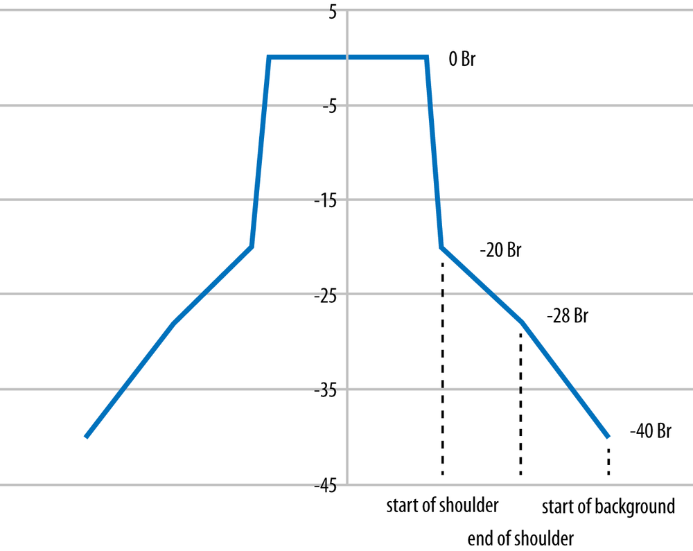
802.11ac channels have exactly the same shape as previous OFDM channels, differing only in the width of the energy transmitted. Figure 2-2 shows the general shape of an 802.11ac channel, which is described as decibels relative (dBr) to the peak level at the channel center frequency. The figure does not label the precise frequencies used because the spectral mask is the same shape no matter what size channel is used. Table 2-2 describes the key points on the spectral mask: the edge of the high-power peak, the start of the shoulder a few megahertz later, the point at which the shoulder steepens, and, finally, the point at which the background is reached.
Available Channel Map
Defining the available channels is more of a regulatory question than a technical one. Wireless LAN equipment is built with flexible radio chips that can tune to almost any frequency, and the 802.11 standards have defined a large number of channels. 802.11ac continues to use the same channel numbering defined by its predecessors, as illustrated in Figure 2-3. The top of the diagram identifies the frequency band and the channel numbers within that band. Channel numbers are spaced four digits apart, but within a wide channel, one of the frequencies is designated as the primary channel; others are called secondary channels. When used as part of an 80 MHz channel, channel 44 may be the primary channel, and channels 36, 40, and 48 will all be secondary channels. Generally speaking, when operating, a wireless LAN will send Beacon frames and announce its existence on its primary channel, but not on its secondary channels. Primary and secondary channels are important to bandwidth coexistence features, and will be discussed further in Clear-Channel Assessment (CCA).
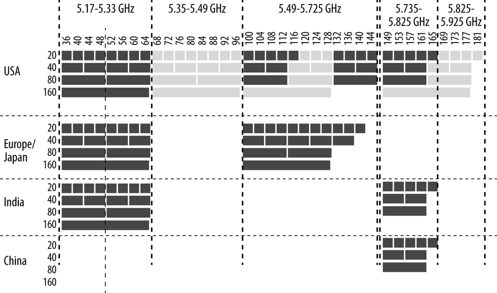
As data has moved from existing wired LANs to wireless networks, additional spectrum has been made available. Regulators are generally aware of the need for additional spectrum, especially to make wider channels available for maximum speeds. The 802.11ac specification defines the channel numbering and layout, but the final say on whether a particular chunk of spectrum can be used lies with the national regulator.
Within Figure 2-3, there is a significant fraction of the spectrum depicted that represents proposed capacity for wireless LANs in the United States. In early 2013, the FCC acted to make a large amount of additional spectrum available. First, it acted to reclaim the “missing” channels between 120 and 128.[10] Second, the FCC moved to allocate two new bands for wireless LAN usage, shown here in the lighter shade, consisting of an additional 195 MHz of spectrum. As you can see from the figure, the FCC action stands to increase the amount of capacity available for 802.11ac by a significant amount. In fact, the proposed commission rules and statements by the commissioners themselves cited 802.11ac as a major driver for allocating this additional spectrum.
Transmission: Modulation, Coding, and Guard Interval
Compared to prior 802.11 specifications, 802.11ac makes only evolutionary improvements to modulation and coding. Compared to its immediate predecessor, 802.11ac simplifies the selection of modulation and coding by discarding the rarely implemented unequal modulation options. Improved modulation technology provides one of the major points where 802.11ac picks up speed. Using the more aggressive 256-QAM modulation lets the link pack in two more bits on each carrier, for a total of eight bits instead of six. Adding two bits increases capacity by a third.
Modulation and Coding Set (MCS)
Selecting a modulation and coding set (MCS) is much simpler in 802.11ac than it was in 802.11n. Rather than the 70-plus options offered by 802.11n, the 802.11ac specification has only 10, shown in Table 2-3. The first seven are mandatory, and most vendors will support 256-QAM, and therefore all nine MCS options, in all products they bring to market. Modulation describes how many bits are contained within one transmission time increment. Higher modulations pack more data into the transmission, but they require much higher signal-to-noise ratios. Like its predecessors, 802.11ac uses an error-correcting code. One of the fundamental attributes of an error-correcting code is that it adds redundant information in a proportion described by the code rate. A code at rate R=1/2 transmits one user data bit (the numerator) for every two bits (the denominator) on the channel. Higher code rates have more data and less redundancy at the cost of not being able to recover from as many errors. In 802.11ac, modulation and coding are coupled together into a single number, the MCS index. Each of the MCS values can lead to a wide range of speeds depending on the channel width, the number of spatial streams, and the guard interval. 802.11ac also does away with unequal modulation, a protocol feature from 802.11n that was not widely implemented.
| MCS index value | Modulation | Code rate (R) |
| 0 | BPSK | 1/2 |
| 1 | QPSK | 1/2 |
| 2 | QPSK | 3/4 |
| 3 | 16-QAM | 1/2 |
| 4 | 16-QAM | 3/4 |
| 5 | 64-QAM | 2/3 |
| 6 | 64-QAM | 3/4 |
| 7 | 64-QAM | 5/6 |
| 8 | 256-QAM | 3/4 |
| 9 | 256-QAM | 5/6 |
One of the ways that 802.11ac simplifies the selection of modulation and coding is that the modulation and coding are no longer tied to the number of spatial streams, as they were in 802.11n. To determine the link speed, knowledge of the MCS must be combined with both the number of streams to produce an overall data rate.
256-QAM modulation
Table 2-3 describes a new modulation for use with 802.11ac. Previous 802.11 standards allowed for up to 64-QAM, which allowed each transmission symbol to take on one of 64 values. At a high level, quadrature amplitude modulation (QAM) works by using the combination of amplitude level and phase shift to select one of many symbols in the constellation. To identify each of the 64 values, there are eight levels of inphase (roughly speaking, a phase shift) and eight levels of quadrature (roughly speaking, the amplitude of a wave). Each time a symbol is transmitted, it may take on one of eight phase shifts and one of eight amplitude levels.[12]
As with many other aspects of the protocol, 802.11ac kicks up the existing technology a notch by using 256-QAM. Rather than a constellation that is 8 by 8, the 256-QAM constellation has 16 phase shifts and 16 amplitude levels. Figure 2-4 compares the 64-QAM constellation to the 256-QAM constellation. At first glance, they’re quite similar, though there are many more constellation points in the latter. One analogy that is often helpful is to compare QAM to a game of darts. The transmitter picks a target point and encodes an amplitude and phase shift. This amplitude and phase shift starts off at the ideal constellation point, and the receiver pulls the transmission out of the air and maps it onto what was received. As the constellation points get closer and closer together, the transmitter must be able to throw its darts much more accurately to hit the target point.
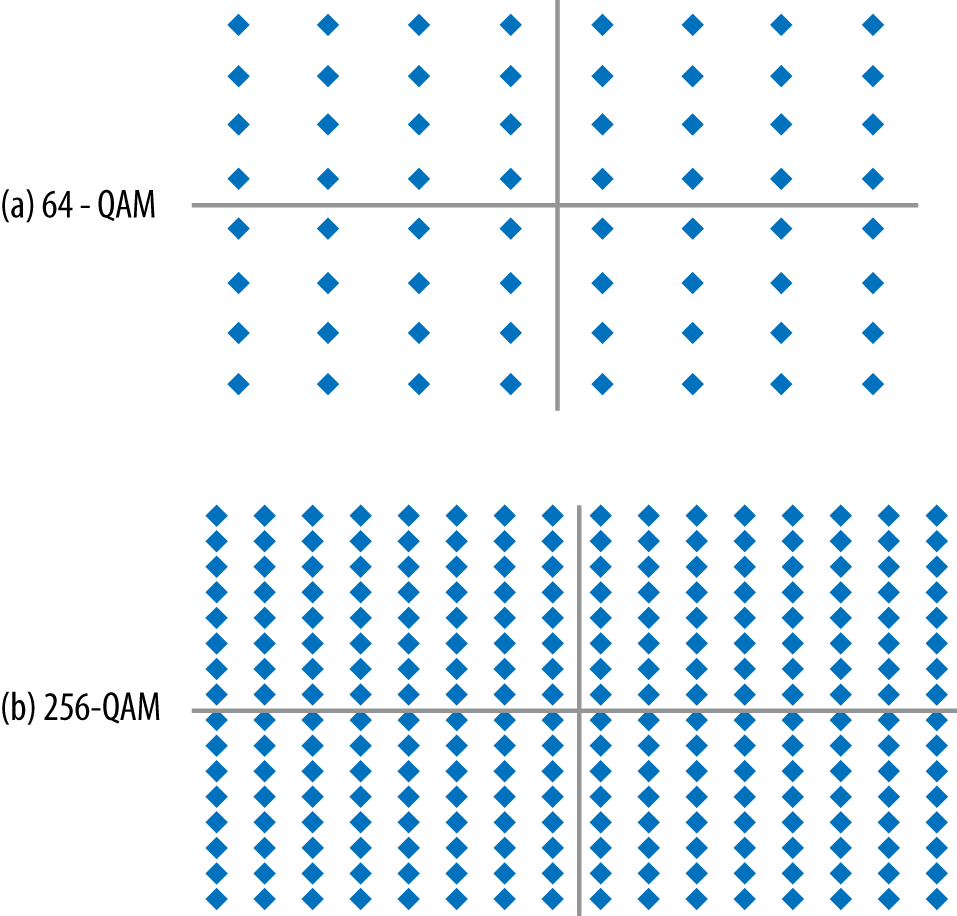
The large number of extra points in the 256-QAM constellation point has the potential to dramatically improve speed. Instead of transmitting a maximum of six bits on each subcarrier in the channel, a 256-QAM-encoded link transmits eight bits. This single feature alone represents a 33% increase in speed over its nearest equivalent in 802.11n.
But nothing comes for free, and the 256-QAM speed boost is no exception. In order to use 256-QAM, the errors in the radio link must be much smaller than before. In a perfect link with ideal transmissions that are received absolutely error-free, the received points line up exactly on the constellation points, and it is easy to understand what should have been transmitted. Real-world radio links are never perfect, though. When a symbol is received, it does not line up exactly on the constellation point. The difference between the ideal constellation point and the point that corresponds to the received symbol exists in two-dimensional space, and therefore the “miss” is described by an error vector, as in Figure 2-5(a). When speaking about a transmission link, generally what system designers are concerned about is the size of the error and not its direction, so it is common to speak of the length of the error, which is called the error vector magnitude (EVM).
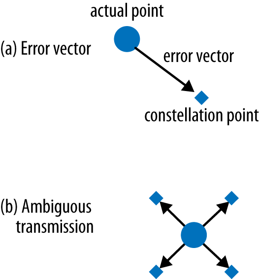
Not surprisingly, transmitting at 256-QAM requires much smaller errors than the less densely packed prior constellations. For example, when the received symbol is in the middle of several constellation points, such as in Figure 2-5(b), the receiver must choose one of the points. If it guesses wrong, the entire frame may need to be discarded. Early implementations of 802.11ac have shown that the required receiver performance for 256-QAM is a gain of about 5 dB over the 64-QAM receiver performance. To achieve better performance, there are a variety of techniques that can be applied. Higher-performance error-correcting codes can provide some of the required performance; 802.11ac includes a low-density parity check (LDPC) code that can provide a gain of 1–2 dB. Selecting better components for the analog frontend on the radio can also help. In addition to any distortions from the ideal point introduced by the radio channel itself, the receiver’s analog section (antenna and amplifier) can also introduce distortion. Minimizing the introduction of errors in the analog section of an 802.11ac interface helps the digital section do its job better. Using LDPC and improving the analog frontend are not mutually exclusive, and some vendors will do both.
Guard Interval
802.11ac retains the ability to select a shortened OFDM guard interval if both the transmitter and the receiver are capable of processing it. With 802.11ac, it has exactly the same effect as in 802.11n: the guard interval shrinks from 800 ns to 400 ns, providing about a 10% boost in throughput. Most 802.11n deployments have proven capable of implementing the short guard interval without difficulty or adverse effects. Although the short guard interval is optional, I expect it to be widely supported, just as it was with 802.11n.[13]
Error-Correcting Codes
802.11ac does not make any changes to the supported error-correcting codes. Convolutional codes are required by 802.11ac, as they have been required for all OFDM PHYs. LDPC coding is supported as an option, and typically offers a gain of 1–2 dB over convolutional coding. Therefore, it is likely to be supported in combination with the very high data rates supported by 256-QAM and long packets transmitted in aggregate frames. By enabling higher data rates, LDPC will also assist in increasing the data rates. An increase in the data rate may enable a reduction in the transmission time, and hence an overall power savings.[14]
PHY-Level Framing
When designing the physical layer framing for 802.11ac, the protocol designers began by laying out requirements that the new frame needed to meet. Most importantly, it needed to be compatible with previous 802.11 PHYs. When an 802.11ac device transmits, 802.11a and 802.11n devices must be able to see and avoid the transmission for the length of time required on the medium. To meet this requirement, the format of the VHT physical layer frame is similar to the mixed-mode format used in 802.11n, and it begins with the same fields as 802.11a frames. A second subtle difference is required to enable multi-user MIMO transmissions, which is that the preamble must be able to describe the number of spatial streams and enable multiple receivers to set up to receive their frames. To meet this second requirement, a new physical layer header was required because the 802.11n HT-SIG header field was not readily extensible to new channel widths or large numbers of spatial streams.
Compared to 802.11n, the physical layer for 802.11ac is much simpler because there is only one format. Figure 2-6 shows the original non-HT format of an OFDM frame in Figure 2-6(a), along with the 802.11n mixed-mode frame format in Figure 2-6(b) and the VHT format in Figure 2-6(c).[15]
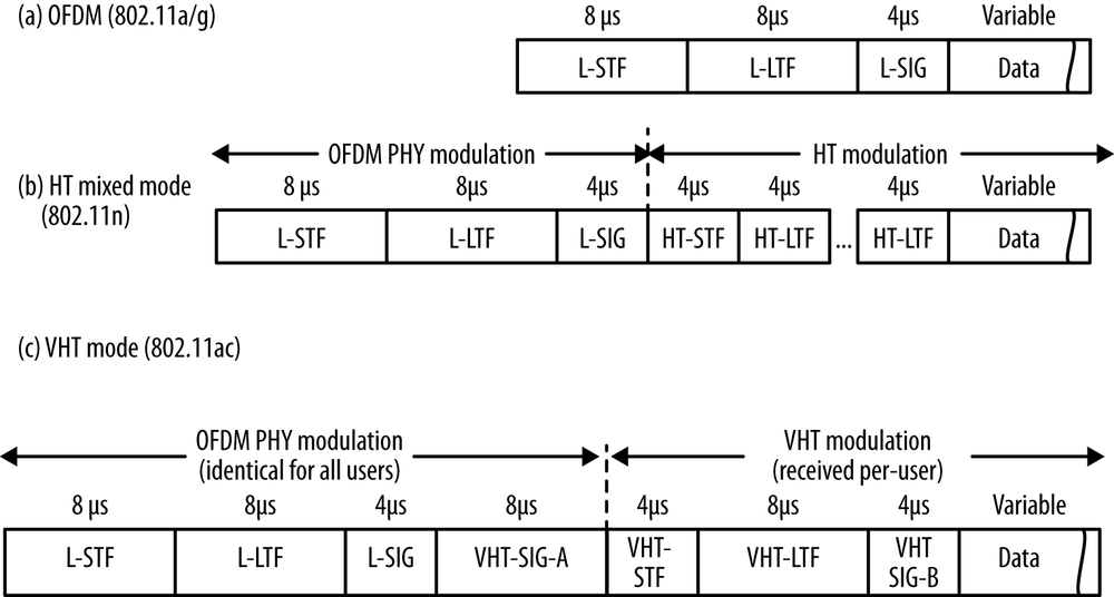
The fields in the VHT frame are as follows:
- Non-HT Short Training Field (L-STF) and Non-HT Long Training Field (L-LTF)
These fields are identical to the fields used in 802.11a; they consist of a sequence of 12 OFDM symbols that are used to assist the receiver in identifying that an 802.11 frame is about to start, synchronizing timers, and selecting an antenna. Any 802.11 device that is capable of OFDM operation can decode these fields.
- Non-HT Signal Field (L-SIG)
The Signal field is used by 802.11a to describe the data rate and length (in bytes) of the frame, which is used by receivers to calculate the time duration of the frame’s transmission. 802.11ac devices set the data rate to 6 Mbps and derive a spoofed length in bytes so that when any receiver calculates its length, it matches the time duration required for the 802.11ac frame.
- VHT Signal A (VHT-SIG-A) and Signal B (VHT-SIG-B) Fields
The VHT Signal fields are the analog of the Signal field used in 802.11a or the HT Signal field used in 802.11n; however, they are understood only by 802.11ac devices. VHT signaling is split into two fields, the Signal A field and its companion, the Signal B field. Taken together, the two fields describe the included frame attributes such as the channel width, modulation and coding, and whether the frame is a single- or multi-user frame. Due to their complexity, these fields are described further in The VHT Signal Fields.
- VHT Short Training Field (VHT-STF)
The VHT STF serves the same purpose as the non-HT STF. Just as the first training fields help a receiver tune in the signal, the VHT-STF assists the receiver in detecting a repeating pattern and setting receiver gain.
- VHT Long Training Field (VHT-LTF)
The VHT long training field consists of a sequence of symbols that set up demodulation of the rest of the frame, starting with the VHT Signal B field. Depending on the number of transmitted streams, it consists of 1, 2, 4, 6, or 8 symbols; the number of required symbols is rounded up to the next highest even numbered value, so a link with five streams would use six symbols. This field’s contents are also used for the channel estimation process that beamforming depends on.
- Data field
The Data field holds the higher-layer protocol packet, or possibly an aggregate frame containing multiple higher-layer packets. This field is described in The Data Field. If no Data field is present in the physical layer payload, it is called a null data packet (NDP), which is used by the VHT PHY for beamforming setup, measurement, and tuning.
Note
Null data packets are physical layer packets, not MAC layer packets. When a physical layer packet has no embedded payload, there is nothing for a MAC analyzer to report.
The VHT Signal Fields
All of the multi-carrier 802.11 PHYs use a Signal field to describe the payload of the physical layer frame, and 802.11ac is no exception. The purpose of the Signal field is to help the receiver decode the data payload, which is done by describing the parameters used for transmission. 802.11ac separates the signal into two different parts, called the Signal A and Signal B fields. The former is in the part of the physical layer header that is received identically by all receivers; the latter is in the part of the physical layer header that is different for each multi-user receiver.
VHT Signal A field
The Signal A field comes first in the frame, and it may take on one of two forms depending on whether the transmission is single-user or multi-user. The depiction of the Signal A field in Figure 2-7 is the format for a single user. (The multi-user format will be discussed in Chapter 4.) Because it holds rate information for decoding the payload of the physical layer frame, it is transmitted with the conservative BPSK modulation with a robust R=1/2 convolutional code. To be intelligible to other stations, it uses the modulation from the 802.11a OFDM PHY, which can transmit 24 bits of data per symbol. The two parts of the VHT Signal A field, each of which corresponds to an OFDM symbol, are referred to as VHT-SIG-A1 and VHT-SIG-A2. The two halves of the field are shown as Figure 2-7(a) and Figure 2-7(b), respectively. To assist a receiver in recognizing that the header belongs to a VHT frame, the constellation rotates between the two symbols.
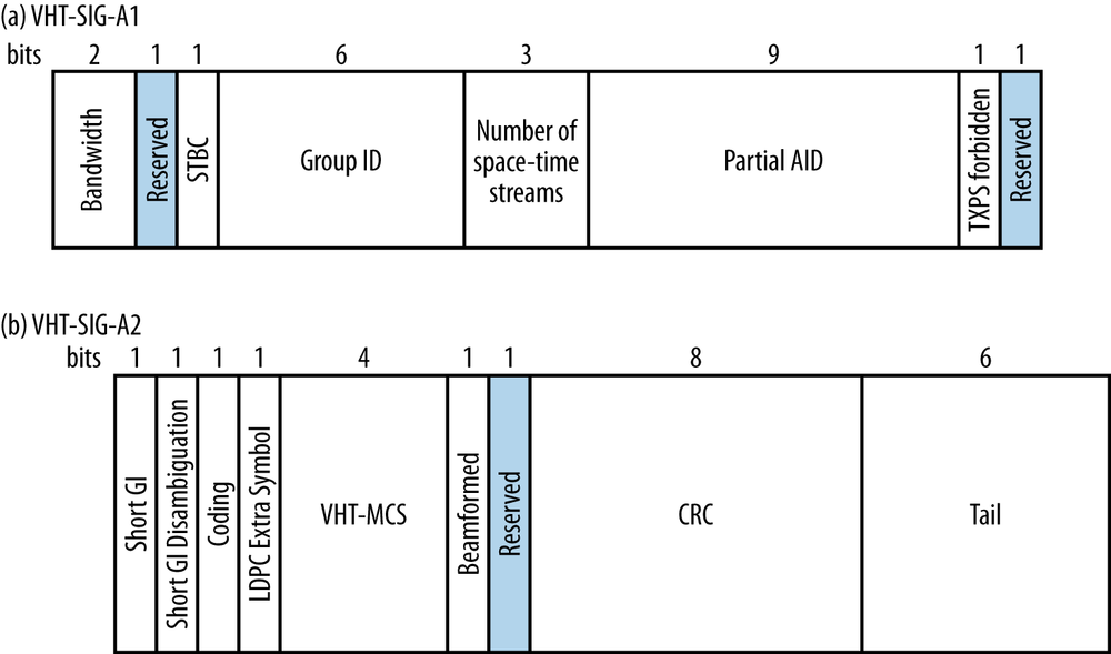
The components of the Signal A field are:
- Bandwidth (2 bits)
Two bits are used to indicate the channel bandwidth: 0 for 20 MHz, 1 for 40 MHz, 2 for 80 MHz, and 3 for 160 MHz.
- STBC (1 bit)
If the payload is encoded with space-time block coding (STBC)[16] for extra robustness, this field will be 1. Otherwise, it will be 0.
- Group ID (6 bits)
When transmitting a single-user frame, this field will be 0 or 63. This field enables a receiver to determine whether the data payload is single- or multi-user. A group ID of 0 is used for frames sent to an AP, and a group ID of 63 is used for frames sent to a client.
- Number of space-time streams (3 bits)
This field indicates the number of space-time streams, but the field is zero-based. Therefore, the number of space-time streams will be one greater than the binary value of this field. For example, if the field is the number 3, then there are four space-time streams.
- Partial AID (9 bits)
For transmissions to an AP, the partial AID is the last nine bits of the BSSID. For a client, the partial AID is an identifier that combines the association ID and the BSSID of its serving AP.
- Transmit power save forbidden (1 bit)
If the access point in a network allows client devices to power off radios when they have the opportunity to transmit frames, this field will be 0. Otherwise, it is 1.
- Short GI (1 bit)
This field is set to 1 to indicate that the 400 ns short guard interval is used for the data payload of the physical layer frame. Otherwise, it is 0.
- Short GI disambiguation (1 bit)
When the short guard interval is used, an extra symbol might be needed for the payload of the physical layer frame. A single bit is used to indicate whether the extra symbol is required (1) or not (0).
- Coding (1 bit)
This field is 0 when convolutional coding is used to protect the Data field, and 1 when LDPC is used.
- LDPC extra symbol (1 bit)
LDPC coding can create the need for an extra OFDM symbol to transmit the Data field. If this field is set to 1, it indicates the extra symbol is required.
- MCS (4 bits)
This field contains the MCS index value for the payload, as shown in the first column of Table 2-3.
- Beamformed (1 bit)
When a beamforming matrix is applied to the transmission, this bit is set to 1; otherwise, it is set to 0.
- CRC (8 bits)
The CRC allows the receiver of the physical layer frame to detect errors in the Signal A field.
- Tail (6 bits)
Six zeros are included to terminate the convolutional coder that protects the Signal A field. Convolutional codes require a “ramp down” of trailing zeros to function properly.
VHT Signal B field
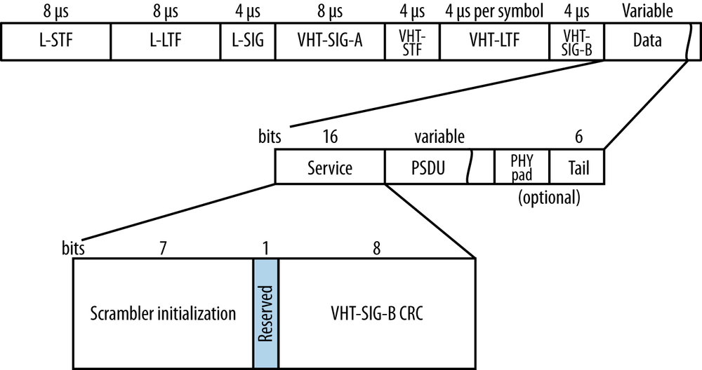
The VHT Signal B field is used to set up the data rate, as well as tune in MIMO reception. Like the VHT Signal A field, it is modulated conservatively to assist receivers in determining the data rate of the payload; however, it is modulated using the VHT MCS 0. Although it is modulated with BPSK with a convolutional code of R=1/2, the VHT modulations have slightly more efficiency and hold a few more bits. The VHT Signal B field is designed to be transmitted in a single OFDM symbol, which is why it has slightly different lengths depending on the channel width. Figure 2-8 shows the single-user format of the VHT Signal B field and its dependence on channel width. (Other formats for this field will be discussed in Chapter 4.)
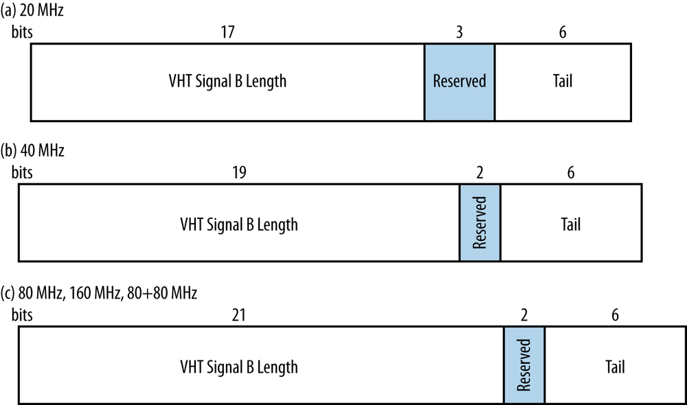
In its single-user form, the raw VHT Signal B field is either 26, 27, or 29 bits, depending on the channel width, and consists of the following fields:
- VHT Signal B Length (17, 19, or 21 bits)
This field measures the length of the Data field payload of the physical layer frame, in four-byte units. This field varies in size so that the maximum value of the field is an approximately constant duration in time (a 40 MHz channel is capable of transmitting much more data in the payload field, and thus needs a longer-length field). The reason why this field measures not the actual number of bytes but the number of four-byte chunks is for efficiency, as will be explained in Frame Size and Aggregation.
- Reserved bits (2 or 3 bits)
The bits between the length field and the tail are reserved, and must be set to 1.
- Tail bits (6 bits)
Six zero bits are included to allow the convolutional coder to complete.
There is no CRC within the VHT Signal B field. To detect errors in the VHT Signal B field, there is a CRC at the start of the Data field, which will be described in the next section.
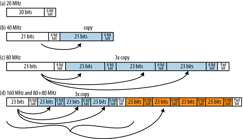
To transmit the VHT Signal B field, it is expanded to fill the available space within one symbol. Wider channels have the capacity to carry more data, so the Signal B field is repeated, as shown in Figure 2-9. For a 40 MHz channel, the field is repeated once. For an 80 MHz channel, the field is repeated three times and a pad bit of 0 is appended. For a 160 MHz (or an 80+80 MHz) channel, the field is repeated four times, a pad bit of 0 is added, and then the resulting structure is repeated once. This process of repeating the signal field ensures that it occupies exactly one symbol.
The Data Field
Immediately following the physical layer header, the Data field begins to transmit the payload of the physical layer frame. The format of the Data field is shown in Figure 2-10. Because the Data field is transmitted following the header, it is transmitted at the data rate described by the physical layer header. The Data field carries a frame from higher protocol layers.
Before beginning transmission of the data from higher-layer protocols, there are a few housekeeping fields embedded in the physical layer frame:
- Service (16 bits)
The Service field is prepended to the higher-level protocol data before transmission. It consists of seven bits to initialize a data scrambler to avoid long runs of identical bits and a CRC of the VHT Signal B field to detect errors.
- PHY Service Data Unit (PSDU), or frame from MAC layer
The PSDU field contains a frame from from the 802.11 MAC layer. It is variable length.
- PHY pad
To ensure that the number of bits passed to the transmitter will exactly match the number of bits required for a symbol, pad bits are added.
- Tail
Tail bits are present when the physical layer frame is protected with a convolutional code and are used to ramp down the convolutional coder. If LDPC is used, the tail bits are not required.
The Transmission and Reception Process
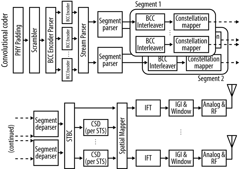
A block diagram for an 802.11ac interface is shown in Figure 2-11. This block diagram can be used to transmit both single-user and multi-user frames, but this chapter focuses on the single-user transmission use case.
When the MAC presents a frame for transmission, it is passed to the physical layer, and the following procedure is run:
Preparation of Service field. To begin, the Service field that is prepended to the data for transmission is constructed. The main component of the Service field is the CRC calculated over the contents of the VHT-SIG-B field.
PHY padding. The first step in transmission is to pad the frame so that its length matches the number of bits required to end on a physical-level symbol boundary.
Scrambling and forward error correction (FEC) encoding. The scrambler reduces the probability of long strings of identical bits in its output, and is present because convolutional codes work best on data that does not have long runs of identical bits. The output of the scrambler is fed to a FEC encoder, which may be either a convolutional coder or an LDPC encoder. To achieve many different code rates, a single-rate FEC encoder’s output may be punctured to achieve higher-rate codes.[17]
Stream parsing. The stream parser takes the output of the FEC encoder and divides up the encoded bits between each spatial stream. For example, if there are two spatial streams, the stream parser will divide up the encoded bits and assign each of them to one of the spatial streams. At this point, the bits flowing from the stream parser to the interleaver are a spatial stream. Output from the stream parser is sent to the interleaver, which is the first component in the radio chain.
Segment parsing. All 160 MHz transmissions, whether using a contiguous 160 MHz block or two 80 MHz blocks, are mapped into two 80 MHz frequency segments. Segment parsing is not performed on 20 MHz, 40 MHz, or 80 MHz transmissions.
Convolutional code interleaving. Convolutional codes work best when errors are isolated, and errors on radio channels tend to affect several bits in a row. The interleaver takes sequential bits from the carriers and separates them in the convolutional code bitstream to separate errors and make them easier to correct. (LDPC has a similar function executed after constellation mapping.)
Constellation mapping. Bits are mapped onto QAM constellation points using the selected modulation. When denser modulations such as 64-QAM or 256-QAM are used, more bits are mapped at a time.
LDPC tone mapping. Tone mapping takes constellation points and ensures they are mapped to OFDM subcarriers separated by a sufficient distance. It serves the same purpose as the interleaver for convolutional codes. For example, in a 40 MHz channel, two consecutive constellation points must be separated by at least six OFDM subcarriers to ensure that interference must be about 1.5 MHz wide to interfere with successive bits.
Segment deparsing. For 160 MHz channels, the segment deparser brings the two frequency segments back together for transformation from constellation symbols into a set of spatial streams suitable for transmission.
Space-time block coding (STBC). This optional step is used to transmit one spatial stream across multiple antennas for extra redundancy. The space-time block coder takes a single constellation symbol output and maps it onto multiple radio chains, transforming the spatial streams into space-time streams.[18]
Pilot insertion and cyclic shift diversity (CSD). Constellation points for transmission are combined with the data for pilot subcarriers to create the complete data set for transmission. When multiple data streams are present, they are each given a small phase shift to aid in distinguishing between them at the receiver. The phase shift is referred to as cyclic shift diversity because a slightly different phase shift is applied to each of the space-time streams.
Spatial mapping. Space-time streams are mapped onto the transmit chains by the spatial mapper. The simplest approach is a direct mapping that turns a spatial stream into a space-time stream for a single transmit chain. For higher performance, the spatial mapper may spread all of the space-time streams on to all of the transmission chains in a spatial expansion. This process is a key component of beamforming, which can be used to shape a space-time stream to direct energy in the direction of a receiver.[19]
Inverse Fourier transform (IFT). An inverse Fourier transform takes frequency-domain data from OFDM and converts it to time-domain data for transmission.
Guard insertion and windowing. The guard interval is inserted at the start of each symbol, and each symbol is windowed to improve signal quality at the receiver.
Preamble construction. The VHT preamble consisting of the non-VHT-modulated training fields (see Figure 2-6(c)) is constructed. The preamble is created for each 20 MHz channel within the transmission channel. To guard against interference, each of the 20 MHz segments of the preamble are given a slight cyclic delay.
RF and analog section. This prepares the data for transmission out an antenna, following the VHT preamble. The complex waveform that comes from the previous step is converted to a signal that can be placed on a carrier at the center frequency of the channel selected by the current AP. A high power amplifier (HPA) increases the power so the signal can travel as far as needed, within regulatory limits.
Receiving frames is the inverse of the transmission process. Incoming signals from the antenna are amplified by a low-noise amplifier (LNA) on each radio chain, and the preamble is used to set up the receiver to adjust for any frequency-specific fades that occur in the channel. After compensating for the channel based on the reception of the preamble and pilot carriers, the incoming data is a series of constellation symbols. If STBC was used for transmission, multiple streams of constellation symbols will be combined into a single output bitstream; otherwise, each space-time stream becomes its own stream of constellation symbols. Constellation symbols are turned into bits and processed by the FEC decoder, which will (hopefully) correct any resulting errors. The resulting bitstream can be descrambled into a MAC frame and passed to the MAC for further processing.
802.11ac Data Rates
Answering the question “How fast does 802.11ac go?” is not straightforward. Data rates are determined by the combination of channel width, modulation and coding, number of spatial streams, and the guard interval. About 5% of 802.11ac draft 2.0 was devoted to tables that answer this question. It’s not useful to create exhaustive tables or complex formulas. Instead, I’ll take it in terms of a few numbers that tend to stick out:
- 400 Mbps (two spatial streams at 40 MHz short guard interval)
This is a full third faster than the comparable 802.11n data rate.
- 900 Mbps (two spatial streams at 80 MHz, short guard interval)
Technically, it’s only 867 Mbps, but it’s nicer to round up and get that much closer to 1 Gbps. I expect the first generation of products will be able to achieve this data rate, though the range at which they will do so is still to be determined.
- 1 Gbps
This isn’t a data rate in the specification itself, but it represents a readily achievable target in high-end equipment. With the same three spatial streams as you get in mainstream 802.11n equipment, you can get to 1.3 Gbps. Or, with four-stream 802.11ac and 80 MHz channels, you can get to 1 Gbps while still using 64-QAM.
802.11ac Data Rate Matrix
Another way to look at the speeds of 802.11ac is to work from a “baseline” speed. At its most basic level, 802.11ac can transmit a single spatial stream in a 20 MHz channel, and the speed of that single spatial stream can be related to many higher data rates through simple mathematical operations. Each spatial stream adds proportionally to throughput. Wider channels also increase throughput proportionally. To get the speed of any MCS rate, take the basic 20 MHz stream, multiply by the number of spatial streams, and then multiply that result by a channel correction factor. Table 2-4 shows how the calculation works. Take the MCS value from the lefthand column, and translate that to the building block data rate in the second column. Multiply by the indicated factors in the next two columns to work out the resulting data rate. The three rightmost columns show the maximum data rates standardized in 802.11ac.
| MCS value | 20 MHz data rate (1SS, short GI) | Spatial stream multiplication factor | Channel width multiplication factor | Maximum 40 MHz rate (8 SS, short GI) | Maximum 80 MHz rate (8 SS, short GI) | Maximum 160 MHz rate (8 SS, short GI) |
| MCS 0 | 7.2 Mbps | x2 for 2 streams x3 for 3 streams x4 for 4 streams x5 for 5 streams x6 for 6 streams x7 for 7 streams x8 for 8 streams | x1.0 for 20 MHz x2.1 for 40 MHz x4.5 for 80 MHz x9.0 for 160 MHz | 120.0 Mbps | 260.0 Mbps | 520.0 Mbps |
| MCS 1 | 14.4 | 240.0 | 520.0 | 1040.0 | ||
| MCS 2 | 21.7 | 360.0 | 780.0 | 1560.0 | ||
| MCS 3 | 28.9 | 480.0 | 1040.0 | 2080.0 | ||
| MCS 4 | 43.3 | 720.0 | 1560.0 | 3120.0 | ||
| MCS 5 | 57.8 | 960.0 | 2080.0 | 4160.0 | ||
| MCS 6 | 65.0 | 1080.0 | 2340.0 | 4680.0 | ||
| MCS 7 | 72.2 | 1200.0 | 2600.0 | 5200.0 | ||
| MCS 8 | 86.7 | 1440.0 | 3120.0 | 6240.0 | ||
| MCS 9 | 96.3[a] | 1600.0 | 3466.7 | 6933.3 | ||
[a] MCS 9 is not allowed for a single stream using a 20 MHz channel, as will be described in the next section. | ||||||
“Missing” MCS values
The 802.11ac standard has several MCS values that are listed as “Not valid” without further explanation, which are listed in Table 2-5. Roughly speaking, these combinations of MCS and channel width do not cleanly fit within the boundaries of the encoding and interleaving process used to assemble a frame.
| 20 MHz | 80 MHz | 160 MHz | |
| MCS 6 | n/a | 3 and 7 SS | n/a |
| MCS 9 | 1, 2, 4, 5, 7, and 8 SS | 6 SS | 3 SS |
To understand why these combinations do not cleanly fit on an encoding boundary, consider the flow of data from higher layers down to symbols, as illustrated in Figure 2-12. Input data first is processed by a forward error correction code. Error-correction codes work by adding redundant bits to recover errors; an R=5/6 code will encode five “data” bits from higher-layer protocols and transmit six “coded” bits. In 802.11ac, multiple encoders each produce an encoding stream, and the output of each encoder is mapped onto each of the subcarrier channels.
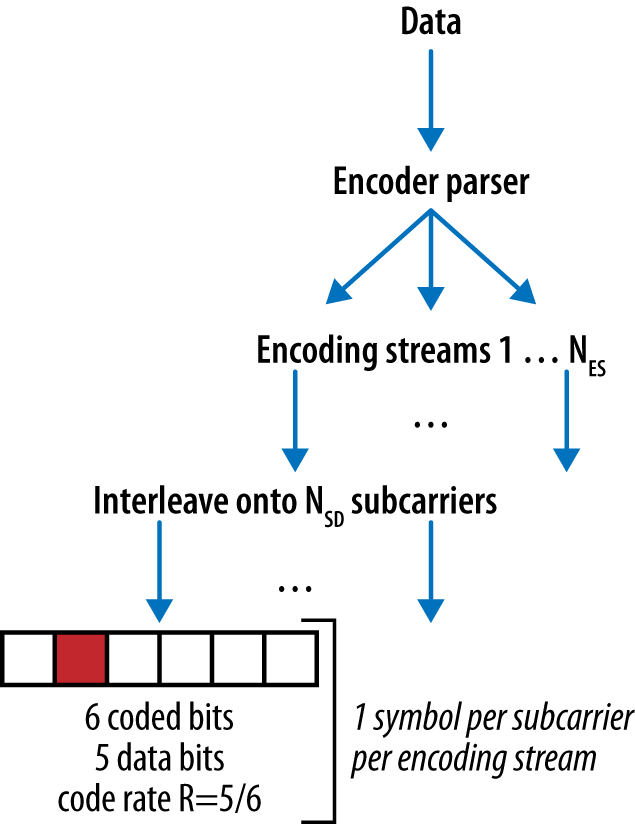
The modulation defines the number of coded bits available per subcarrier. With 256-QAM operating on a 20 MHz channel, for example, there are 416 coded bits available per subcarrier. When the code rate is 3/4, as in MCS 8, the 416 coded bits are broken up into 104 blocks. When the code rate is 5/6, however, the 416 coded bits do not cleanly break into a series of blocks. There are 69 blocks of 6 bits, with 2 bits left over. The 802.11ac task group elected not to add padding, and simply listed the resulting data rate as not valid.
Roughly speaking, the rule for determining whether an MCS will be valid is that the number of coded bits per subcarrier must be an integer multiple of the number of encoding streams. Furthermore, the number of coded bits per encoding stream must be an integer multiple of the denominator in the code rate.[20]
Comparison of 802.11ac Data Rates to Other 802.11 PHYs
For another view, see Table 2-6, which compares the highest possible data rate for several wireless technology combinations. The table compares the top data rate, not necessarily a typical data rate. 802.11ac speeds are quoted using 256-QAM, which may not always be achievable in real-world deployments.
| Technology | 20 MHz[a] | 40 MHz | 80 MHz | 160 MHz |
| 802.11b | 11 Mbps | |||
| 802.11a/g | 54 Mbps | |||
| 802.11n (1 SS) | 72 Mbps | 150 Mbps | ||
| 802.11ac (1 SS) | 87 Mbps | 200 Mbps | 433 Mbps | 867 Mbps |
| 802.11n (2 SS) | 144 Mbps | 300 Mbps | ||
| 802.11ac (2 SS) | 173 Mbps | 400 Mbps | 867 Mbps | 1.7 Gbps |
| 802.11n (3 SS) | 216 Mbps | 450 Mbps | ||
| 802.11ac (3 SS) | 289 Mbps | 600 Mbps | 1.3 Gbps | 2.3 Gbps[b] |
| 802.11n (4 SS)[c] | 289 Mbps | 600 Mbps | ||
| 802.11ac (4 SS) | 347 Mbps | 800 Mbps | 1.7 Gbps | 3.5 Gbps |
| 802.11ac (8 SS) | 693 Mbps | 1.6 Gbps | 3.4 Gbps | 6.9 Gbps |
[a] MCS 9 is not valid for 802.11ac in 20 MHz channels, so the 20 MHz values for 802.11ac are MCS 8. [b] MCS 9 is not valid for a three-stream 802.11ac device with 160 MHz channels, so this is the (lower) value for MCS 8. [c] Four-stream 802.11n products were never released widely. I expect the market to leapfrog four-stream 11n for four-stream 11ac; this line in the table is included for comparison purposes. | ||||
Mandatory PHY Features
802.11ac is a complex specification with a large number of protocol features. Table 2-7 classifies the protocol features as either mandatory or optional. As a general principle, the Wi-Fi Alliance certification programs validate mandatory functionality in the specification, and create optional tests only for the most widely supported and high-value features.
| Feature | Mandatory/Optional | Comments |
| Support for VHT format of frames | Mandatory | |
| 20 & 40 MHz channels | Mandatory | These channel widths were required in previous PHY standards. |
| 80 MHz channels | Mandatory | |
| 160 MHz and 80+80 MHz operation | Optional | Not supported by first wave of devices. |
| Single-stream operation MCS 0 through 7 | Mandatory | |
| Single-stream operation MCS 8 and 9 | Optional | Optional, but likely to be widely supported. |
| Two-stream operation | Optional | Mandatory in WFA program for anything other than a battery-operated mobile AP, just as with 802.11n certification. |
| Three-stream operation | Optional | |
| Four-stream operation | Optional | |
| Five- to eight-stream operation | Optional | Not likely to be supported until later product releases. |
| Support for MCS 8 and 9 (256-QAM) with more than one stream | Optional | |
| Short guard interval of 400 ns | Optional | Although optional, this will be widely supported. (Approximately 3/4 of WFA-certified 11n devices implement the feature.) |
| LDPC | Optional | Likely to be supported in tandem with 256-QAM. |
| STBC | Optional | Likely to be moderately well supported, but most products will implement only single-stream (2x1) operation. |
[9] As you will see in Chapter 4, this is an (intentionally) simplified description of MIMO transmission. A single data stream does not necessarily follow a single clean, linear path through space, in large part due to the dependence of transmission on frequency.
[10] Within the 5.47–5.725 GHz band, wireless LANs are considered “secondary” users, meaning they must avoid interfering with the primary band users. One of the primary band users is Terminal-area Doppler Weather Radar (TDWR) at 5.600–5.650 GHz, a technology that monitors airport approaches for hazardous wind shear conditions. In 1985, Delta Air Lines flight 191 crashed after flying through storms. The crash directly led to onboard wind shear detection and the development of TDWR to assist pilots and air traffic controllers in avoiding these conditions. For more information, see my blog post on why we lost the weather radar channels.
[11] The Commission action to propose rules for this new spectrum, numbered FCC 13-22, is available at the FCC website.
[12] There is a bit more to QAM than saying that it uses phase shifts and amplitude levels, but if you want to know the details, you are probably in a hardware engineering class or are a chip designer.
[13] For more information on the short guard interval, see Chapter 3 of 802.11n: A Survival Guide.
[14] For more information on error-correcting codes, see Chapter 3 of 802.11n: A Survival Guide.
[15] For more information about the HT frame formats in 802.11n, see Chapter 3 of 802.11n: A Survival Guide.
[16] STBC may be used when the number of radio chains exceeds the number of spatial streams; it transmits a single data stream across two spatial streams. In effect, it takes MIMO gain and translates it into increased range.
[17] For more information on puncturing, see Chapter 13 of 802.11 Wireless Networks: The Definitive Guide.
[18] For more information on STBC, see Chapter 4 of 802.11n: A Survival Guide.
[19] A spatial expansion takes a given number of space-time streams and maps them onto transmit chains by using a matrix multiplication. Because the matrix multiplication can affect how much energy is directed from each transmission chain, the matrix is sometimes called a steering matrix when it is used to direct beam energy.
[20] For the full details, see slide 4 of 802.11 document 11-10/0820r0, which lays out the framework for MCS selection, and 802.11 document 11-11/0577r1, which proposed filling in some of the data rate holes in 802.11ac by increasing the number of encoders within products.
Get 802.11ac: A Survival Guide now with the O’Reilly learning platform.
O’Reilly members experience books, live events, courses curated by job role, and more from O’Reilly and nearly 200 top publishers.

