Chapter 1. Big Data Technology Primer
Apache Hadoop is a tightly integrated ecosystem of different software products built to provide scalable and reliable distributed storage and distributed processing. The inspiration for much of the Hadoop ecosystem was a sequence of papers published by Google in the 2000s, describing innovations in systems to produce reliable storage (the Google File System), processing (MapReduce, Pregel), and low-latency random-access queries (Bigtable) on hundreds to thousands of potentially unreliable servers. For Google, the primary driver for developing these systems was pure expediency: there simply were no technologies at the time capable of storing and processing the vast datasets it was dealing with. The traditional approach to performing computations on datasets was to invest in a few extremely powerful servers with lots of processors and lots of RAM, slurp the data in from a storage layer (e.g., NAS or SAN), crunch through a computation, and write the results back to storage. As the scale of the data increased, this approach proved both impractical and expensive.
The key innovation, and one which still stands the test of time, was to distribute the datasets across many machines and to split up any computations on that data into many independent, “shared-nothing” chunks, each of which could be run on the same machines storing the data. Although existing technologies could be run on multiple servers, they typically relied heavily on communication between the distributed components, which leads to diminishing returns as the parallelism increases (see Amdahl’s law). By contrast, in the distributed-by-design approach, the problem of scale is naturally handled because each independent piece of the computation is responsible for just a small chunk of the dataset. Increased storage and compute power can be obtained by simply adding more servers—a so-called horizontally scalable architecture. A key design point when computing at such scales is to design with the assumption of component failure in order to build a reliable system from unreliable components. Such designs solve the problem of cost-effective scaling because the storage and computation can be realized on standard commodity servers.
Note
With advances in commodity networking and the general move to cloud computing and storage, the requirement to run computations locally to the data is becoming less critical. If your network infrastructure is good enough, it is no longer essential to use the same underlying hardware for compute and storage. However, the distributed nature and horizontally scalable approach are still fundamental to the efficient operation of these systems.
Hadoop is an open source implementation of these techniques. At its core, it offers a distributed filesystem (HDFS) and a means of running processes across a cluster of servers (YARN). The original distributed processing application built on Hadoop was MapReduce, but since its inception, a wide range of additional software frameworks and libraries have grown up around Hadoop, each one addressing a different use case. In the following section, we go on a whirlwind tour of the core technologies in the Hadoop project, as well as some of the more popular open source frameworks in the ecosystem that run on Hadoop clusters.
A Tour of the Landscape
When we say “Hadoop,” we usually really mean Hadoop and all the data engineering projects and frameworks that have been built around it. In this section, we briefly review a few key technologies, categorized by use case. We are not able to cover every framework in detail—in many cases these have their own full book-level treatments—but we try to give a sense of what they do. This section can be safely skipped if you are already familiar with these technologies, or you can use it as a handy quick reference to remind you of the fundamentals.
The zoo of frameworks, and how they relate to and depend on each other, can appear daunting at first, but with some familiarization, the relationships become clearer. You may have seen representations similar to Figure 1-2, which attempt to show how different components build on each other. These diagrams can be a useful aid to understanding, but they don’t always make all the dependencies among projects clear. Projects depend on each other in different ways, but we can think about two main types of dependency: data and control. In the data plane, a component depends on another component when reading and writing data, while in the control plane, a component depends on another component for metadata or coordination. For the graphically inclined, some of these relationships are shown in Figure 1-3. Don’t panic; this isn’t meant to be scary, and it’s not critical at this stage that you understand exactly how the dependencies work between the components. But the graphs demonstrate the importance of developing a basic understanding of the purpose of each element in the stack. The aim of this section is to give you that context.

Figure 1-2. Standard representation of technologies and dependencies in the Hadoop stack
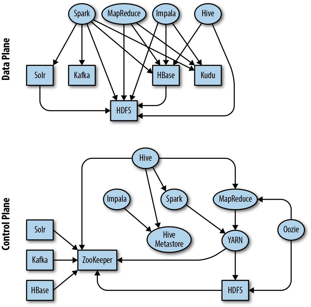
Figure 1-3. Graphical representation of some dependencies between components in the data and control planes
Note
Where there are multiple technologies with a similar design, architecture, and use case, we cover just one but strive to point out the alternatives as much as possible, either, in the text or in “Also consider” sections.
Core Components
The first set of projects are those that form the core of the Hadoop project itself or are key enabling technologies for the rest of the stack: HDFS, YARN, Apache ZooKeeper, and the Apache Hive Metastore. Together, these projects form the foundation on which most other frameworks, projects, and applications running on the cluster depend.
HDFS
The Hadoop Distributed File System (HDFS) is the scalable, fault-tolerant, and distributed filesystem for Hadoop. Based on the original use case of analytics over large-scale datasets, HDFS is optimized to store very large amounts of immutable data with files being typically accessed in long sequential scans. HDFS is the critical supporting technology for many of the other components in the stack.
When storing data, HDFS breaks up a file into blocks of configurable size, usually something like 128 MiB, and stores a replica of each block on multiple servers for resilience and data parallelism. Each worker node in the cluster runs a daemon called a DataNode which accepts new blocks and persists them to its local disks. The DataNode is also responsible for serving up data to clients. The DataNode is only aware of blocks and their IDs; it does not have knowledge about the file to which a particular replica belongs. This information is curated by a coordinating process, the NameNode, which runs on the master servers and is responsible for maintaining a mapping of files to the blocks, as well as metadata about the files themselves (things like names, permissions, attributes, and replication factor).
Clients wishing to store blocks must first communicate with the NameNode to be given a list of DataNodes on which to write each block. The client writes to the first DataNode, which in turn streams the data to the next DataNode, and so on in a pipeline. When providing a list of DataNodes for the pipeline, the NameNode takes into account a number of things, including available space on the DataNode and the location of the node—its rack locality. The NameNode insures against node and rack failures by ensuring that each block is on at least two different racks. In Figure 1-4, a client writes a file consisting of three blocks to HDFS, and the process distributes and replicates the data across DataNodes.
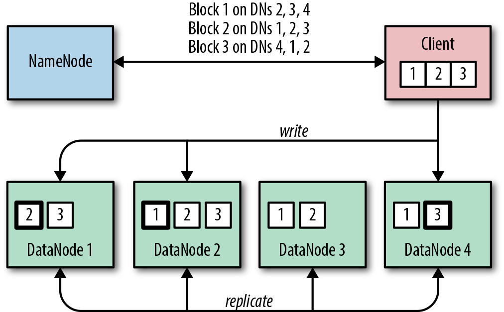
Figure 1-4. The HDFS write process and how blocks are distributed across DataNodes
Likewise, when reading data, the client asks the NameNode for a list of DataNodes containing the blocks for the files it needs. The client then reads the data directly from the DataNodes, preferring replicas that are local or close, in network terms.
The design of HDFS means that it does not allow in-place updates to the files it stores. This can initially seem quite restrictive until you realize that this immutability allows it to achieve the required horizontal scalability and resilience in a relatively simple way.
HDFS is fault-tolerant because the failure of an individual disk, DataNode, or even rack does not imperil the safety of the data. In these situations, the NameNode simply directs one of the DataNodes that is maintaining a surviving replica to copy the block to another DataNode until the required replication factor is reasserted. Clients reading data are directed to one of the remaining replicas. As such, the whole system is self-healing, provided we allow sufficient capacity and redundancy in the cluster itself.
HDFS is scalable, given that we can simply increase the capacity of the filesystem by adding more DataNodes with local storage. This also has the nice side effect of increasing the available read and write throughput available to HDFS as a whole.
It is important to note, however, that HDFS does not achieve this resilience and scaling all on its own. We have to use the right servers and design the layout of our clusters to take advantage of the resilience and scalability features that HDFS offers—and in large part, that is what this book is all about. In Chapter 3, we discuss in detail how HDFS interacts with the servers on which its daemons run and how it uses the locally attached disks in these servers. In Chapter 4, we examine the options when putting a network plan together, and in Chapter 12, we cover how to make HDFS as highly available and fault-tolerant as possible.
One final note before we move on. In this short description of HDFS, we glossed over the fact that Hadoop abstracts much of this detail from the client. The API that a client uses is actually a Hadoop-compatible filesystem, of which HDFS is just one implementation. We will come across other commonly used implementations in this book, such as cloud-based object storage offerings like Amazon S3.
YARN
Although it’s useful to be able to store data in a scalable and resilient way, what we really want is to be able to derive insights from that data. To do so, we need to be able to compute things from the data, in a way that can scale to the volumes we expect to store in our Hadoop filesystem. What’s more, we need to be able to run lots of different computations at the same time, making efficient use of the available resources across the cluster and minimizing the required effort to access the data. Each computation processes different volumes of data and requires different amounts of compute power and memory. To manage these competing demands, we need a centralized cluster manager, which is aware of all the available compute resources and the current competing workload demands.
This is exactly what YARN (Yet Another Resource Negotiator) is designed to be. YARN runs a daemon on each worker node, called a NodeManager, which reports in to a master process, called the ResourceManager. Each NodeManager tells the ResourceManager how much compute resource (in the form of virtual cores, or vcores) and how much memory is available on its node. Resources are parceled out to applications running on the cluster in the form of containers, each of which has a defined resource demand—say, 10 containers each with 4 vcores and 8 GB of RAM. The NodeManagers are responsible for starting and monitoring containers on their local nodes and for killing them if they exceed their stated resource allocations.
An application that needs to run computations on the cluster must first ask the ResourceManager for a single container in which to run its own coordination process, called the ApplicationMaster (AM). Despite its name, the AM actually runs on one of the worker machines. ApplicationMasters of different applications will run on different worker machines, thereby ensuring that a failure of a single worker machine will affect only a subset of the applications running on the cluster. Once the AM is running, it requests additional containers from the ResourceManager to run its actual computation. This process is sketched in Figure 1-5: three clients run applications with different resource demands, which are translated into different-sized containers and spread across the NodeManagers for execution.
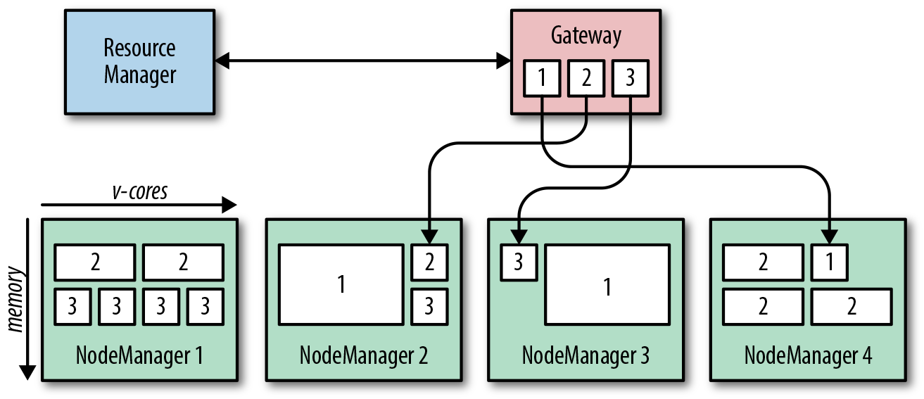
Figure 1-5. YARN application execution.
The ResourceManager runs a special thread, which is responsible for scheduling application requests and ensuring that containers are allocated equitably between applications and users running applications on the cluster. This scheduler strives to allocate cores and memory fairly between tenants. Tenants and workloads are divided into hierarchical pools, each of which has a configurable share of the overall cluster resources.
It should be clear from the description that YARN itself does not perform any computation but rather is a framework for launching such applications distributed across a cluster. YARN provides a suite of APIs for creating these applications; we cover two such implementations, MapReduce and Apache Spark, in “Computational Frameworks”.
You’ll learn more about making YARN highly available in Chapter 12.
Apache ZooKeeper
The problem of consensus is an important topic in computer science. When an application is distributed across many nodes, a key concern is getting these disparate components to agree on the values of some shared parameters. For example, for frameworks with multiple master processes, agreeing on which process should be the active master and which should be in standby is critical to their correct operation.
Apache ZooKeeper is the resilient, distributed configuration service for the Hadoop ecosystem. Within ZooKeeper, configuration data is stored and accessed in a filesystem-like tree of nodes, called znodes, each of which can hold data and be the parent of zero or more child nodes. Clients open a connection to a single ZooKeeper server to create, read, update and delete the znodes.
For resilience, ZooKeeper instances should be deployed on different servers as an ensemble. Since ZooKeeper operates on majority consensus, an odd number of servers is required to form a quorum. Although even numbers can be deployed, the extra server provides no extra resilience to the ensemble. Each server is identical in functionality, but one of the ensemble is elected as the leader node—all other servers are designated followers. ZooKeeper guarantees that data updates are applied by a majority of ZooKeeper servers. As long as a majority of servers are up and running, the ensemble is operational. Clients can open connections to any of the servers to perform reads and writes, but writes are forwarded from follower servers to the leader to ensure consistency. ZooKeeper ensures that all state is consistent by guaranteeing that updates are always applied in the same order.
Tip
In general, a quorum with n members can survive up to floor((n–1)/2) failures and still be operational. Thus, a four-member ensemble has the same resiliency properties as an ensemble of three members.
As outlined in Table 1-1, many frameworks in the ecosystem rely on ZooKeeper for maintaining highly available master processes, coordinating tasks, tracking state, and setting general configuration parameters. You’ll learn more about how ZooKeeper is used by other components for high availability in Chapter 12.
| Project | Usage of ZooKeeper |
|---|---|
HDFS |
Coordinating high availability |
HBase |
Metadata and coordination |
Solr |
Metadata and coordination |
Kafka |
Metadata and coordination |
YARN |
Coordinating high availability |
Hive |
Table and partition locking and high availability |
Apache Hive Metastore
We’ll cover the querying functionality of Apache Hive in a subsequent section when we talk about analytical SQL engines, but one component of the project—the Hive Metastore—is such a key supporting technology for other components of the stack that we need to introduce it early on in this survey.
The Hive Metastore curates information about the structured datasets (as opposed to unstructured binary data) that reside in Hadoop and organizes them into a logical hierarchy of databases, tables, and views. Hive tables have defined schemas, which are specified during table creation. These tables support most of the common data types that you know from the relational database world. The underlying data in the storage engine is expected to match this schema, but for HDFS this is checked only at runtime, a concept commonly referred to as schema on read. Hive tables can be defined for data in a number of storage engines, including Apache HBase and Apache Kudu, but by far the most common location is HDFS.
In HDFS, Hive tables are nothing more than directories containing files. For large tables, Hive supports partitioning via subdirectories within the table directory, which can in turn contain nested partitions, if necessary. Within a single partition, or in an unpartitioned table, all files should be stored in the same format; for example, comma-delimited text files or a binary format like Parquet or ORC. The metastore allows tables to be defined as either managed or external. For managed tables, Hive actively controls the data in the storage engine: if a table is created, Hive builds the structures in the storage engine, for example by making directories on HDFS. If a table is dropped, Hive deletes the data from the storage engine. For external tables, Hive makes no modifications to the underlying storage engine in response to metadata changes, but merely maintains the metadata for the table in its database.
Other projects, such as Apache Impala and Apache Spark, rely on the Hive Metastore as the single source of truth for metadata about structured datasets within the cluster. As such it is a critical component in any deployment.
Going deeper
There are some very good books on the core Hadoop ecosystem, which are well worth reading for a thorough understanding. In particular, see:
-
Hadoop: The Definitive Guide, 4th Edition, by Tom White (O’Reilly)
-
ZooKeeper, by Benjamin Reed and Flavio Junqueira (O’Reilly)
-
Programming Hive, by Dean Wampler, Jason Rutherglen, and Edward Capriolo (O’Reilly)
Computational Frameworks
With the core Hadoop components, we have data stored in HDFS and a means of running distributed applications via YARN. Many frameworks have emerged to allow users to define and compose arbitrary computations and to allow these computations to be broken up into smaller chunks and run in a distributed fashion. Let’s look at two of the principal frameworks.
Hadoop MapReduce
MapReduce is the original application for which Hadoop was built and is a Java-based implementation of the blueprint laid out in Google’s MapReduce paper. Originally, it was a standalone framework running on the cluster, but it was subsequently ported to YARN as the Hadoop project evolved to support more applications and use cases. Although superseded by newer engines, such as Apache Spark and Apache Flink, it is still worth understanding, given that many higher-level frameworks compile their inputs into MapReduce jobs for execution. These include:
-
Apache Hive
-
Apache Sqoop
-
Apache Oozie
-
Apache Pig
Note
The terms map and reduce are borrowed from functional programming, where a map applies a transform function to every element in a collection, and a reduce applies an aggregation function to each element of a list, combining them into fewer summary values.
Essentially, MapReduce divides a computation into three sequential stages: map, shuffle, and reduce. In the map phase, the relevant data is read from HDFS and processed in parallel by multiple independent map tasks. These tasks should ideally run wherever the data is located—usually we aim for one map task per HDFS block. The user defines a map() function (in code) that processes each record in the file and produces key-value outputs ready for the next phase. In the shuffle phase, the map outputs are fetched by MapReduce and shipped across the network to form input to the reduce tasks. A user-defined reduce() function receives all the values for a key in turn and aggregates or combines them into fewer values which summarize the inputs. The essentials of the process are shown in Figure 1-6. In the example, files are read from HDFS by mappers and shuffled by key according to an ID column. The reducers aggregate the remaining columns and write the results back to HDFS.
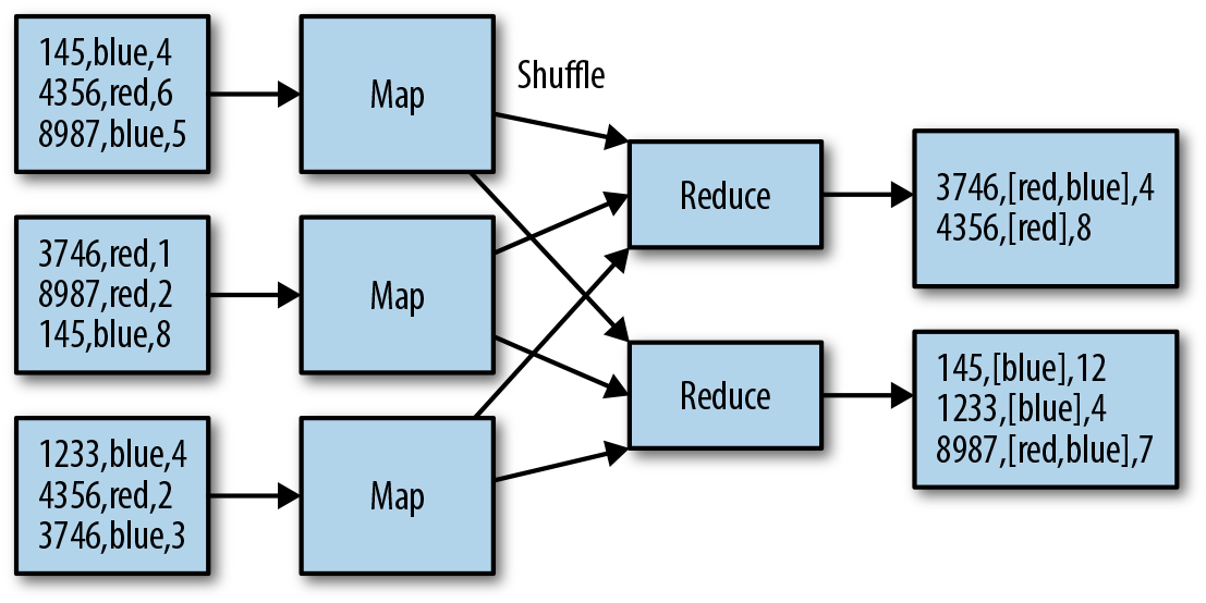
Figure 1-6. Simple aggregation performed in MapReduce
Sequences of these three simple linear stages can be composed and combined into essentially any computation of arbitrary complexity; for example, advanced transformations, joins, aggregations, and more. Sometimes, for simple transforms that do not require aggregations, the reduce phase is not required at all. Usually, the outputs from a MapReduce job are stored back into HDFS, where they may form the inputs to other jobs.
Despite its simplicity, MapReduce is incredibly powerful and extremely robust and scalable. It does have a couple of drawbacks, though. First, it is quite involved from the point of view of a user, who needs to code and compile map() and reduce() functions in Java, which is too high a bar for many analysts—composing complex processing pipelines in MapReduce can be a daunting task. Second, MapReduce itself is not particularly efficient. It does a lot of disk-based I/O, which can be expensive when combining processing stages together or doing iterative operations. Multistage pipelines are composed from individual MapReduce jobs with an HDFS I/O barrier in between, with no recognition of potential optimizations in the whole processing graph.
Because of these drawbacks, a number of successors to MapReduce have been developed that aim both to simplify development and to make processing pipelines more efficient. Despite this, the conceptual underpinnings of MapReduce—that data processing should be split up into multiple independent tasks running on different machines (maps), the results of which are then shuffled to and grouped and collated together on another set of machines (reduces)—are fundamental to all distributed data processing engines, including SQL-based frameworks. Apache Spark, Apache Flink, and Apache Impala, although all quite different in their specifics, are all essentially different implementations of this concept.
Apache Spark
Apache Spark is a distributed computation framework, with an emphasis on efficiency and usability, which supports both batch and streaming computations. Instead of the user having to express the necessary data manipulations in terms of pure map() and reduce() functions as in MapReduce, Spark exposes a rich API of common operations, such as filtering, joining, grouping, and aggregations directly on Datasets, which comprise rows all adhering to a particular type or schema. As well as using API methods, users can submit operations directly using a SQL-style dialect (hence the general name of this set of features, Spark SQL), removing much of the requirement to compose pipelines programmatically. With its API, Spark makes the job of composing complex processing pipelines much more tractable to the user. As a simple example, in Figure 1-7, three datasets are read in. Two of these unioned together and joined with a third, filtered dataset. The result is grouped according to a column and aggregated and written to an output. The dataset sources and sinks could be batch-driven and use HDFS or Kudu, or could be processed in a stream to and from Kafka.
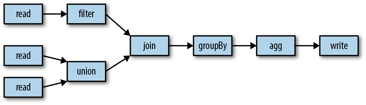
Figure 1-7. A typical simple aggregation performed in Spark
A key feature of operations on datasets is that the processing graphs are run through a standard query optimizer before execution, very similar to those found in relational databases or in massively parallel processing query engines. This optimizer can rearrange, combine, and prune the processing graph to obtain the most efficient execution pipeline. In this way, the execution engine can operate on datasets in a much more efficient way, avoiding much of the intermediate I/O from which MapReduce suffers.
One of the principal design goals for Spark was to take full advantage of the memory on worker nodes, which is available in increasing quantities on commodity servers. The ability to store and retrieve data from main memory at speeds which are orders of magnitude faster than those of spinning disks makes certain workloads radically more efficient. Distributed machine learning workloads in particular, which often operate on the same datasets in an iterative fashion, can see huge benefits in runtimes over the equivalent MapReduce execution. Spark allows datasets to be cached in memory on the executors; if the data does not fit entirely into memory, the partitions that cannot be cached are spilled to disk or transparently recomputed at runtime.
Spark implements stream processing as a series of periodic microbatches of datasets. This approach requires only minor code differences in the transformations and actions applied to the data—essentially, the same or very similar code can be used in both batch and streaming modes. One drawback of the micro-batching approach is that it takes at least the interval between batches for an event to be processed, so it is not suitable for use cases requiring millisecond latencies. However, this potential weakness is also a strength because microbatching allows much greater data throughput than can be achieved when processing events one by one. In general, there are relatively few streaming use cases that genuinely require subsecond response times. However, Spark’s structured streaming functionality promises to bring many of the advantages of an optimized Spark batch computation graph to a streaming context, as well as a low-latency continuous streaming mode.
Spark ships a number of built-in libraries and APIs for machine learning. Spark MLlib allows the process of creating a machine learning model (data preparation, cleansing, feature extraction, and algorithm execution) to be composed into a distributed pipeline. Not all machine learning algorithms can automatically be run in a distributed way, so Spark ships with a few implementations of common classes of problems, such as clustering, classification and regression, and collaborative filtering.
Spark is an extraordinarily powerful framework for data processing and is often (rightly) the de facto choice when creating new batch processing, machine learning, and streaming use cases. It is not the only game in town, though; application architects should also consider options like Apache Flink for batch and stream processing, and Apache Impala (see “Apache Impala”) for interactive SQL.
Going deeper
Once again, Hadoop: The Definitive Guide, by Tom White, is the best resource to learn more about Hadoop MapReduce. For Spark, there are a few good references:
-
Spark: The Definitive Guide, by Bill Chambers and Matei Zaharia (O’Reilly)
-
High Performance Spark, by Holden Karau and Rachel Warren (O’Reilly)
Analytical SQL Engines
Although MapReduce and Spark are extremely flexible and powerful frameworks, to use them you do need to be comfortable programming in a language like Java, Scala, or Python and should be happy deploying and running code from the command line. The reality is that, in most enterprises, SQL remains the lingua franca of analytics, and the largest, most accessible skill base lies there. Sometimes you need to get things done without the rigmarole of coding, compiling, deploying, and running a full application. What’s more, a large body of decision support and business intelligence tools interact with data stores exclusively over SQL. For these reasons, a lot of time and effort has been spent developing SQL-like interfaces to structured data stored in Hadoop. Many of these use MapReduce or Spark as their underlying computation mechanism, but some are computation engines in their own right. Each engine is focused on querying data that already exists in the storage engine or on inserting new data in bulk into those engines. They are designed for large-scale analytics and not for small-scale transactional processing. Let’s look at the principal players.
Apache Hive
Apache Hive is the original data warehousing technology for Hadoop. It was developed at Facebook and was the first to offer a SQL-like language, called HiveQL, to allow analysts to query structured data stored in HDFS without having to first compile and deploy code. Hive supports common SQL query concepts, like table joins, unions, subqueries, and views. At a high level, Hive parses a user query, optimizes it, and compiles it into one or more chained batch computations, which it runs on the cluster. Typically these computations are executed as MapReduce jobs, but Hive can also use Apache Tez and Spark as its backing execution engine. Hive has two main components: a metadata server and a query server. We covered the Hive Metastore earlier, so we focus on the querying functionality in this section.
Users who want to run SQL queries do so via the query server, called HiveServer2 (HS2). Users open sessions with the query server and submit queries in the HQL dialect. Hive parses these queries, optimizes them as much as possible, and compiles them into one or more batch jobs. Queries containing subqueries get compiled into multistage jobs, with intermediate data from each stage stored in a temporary location on HDFS. HS2 supports multiple concurrent user sessions and ensures consistency via shared or exclusive locks in ZooKeeper. The query parser and compiler uses a cost-based optimizer to build a query plan and can use table and column statistics (which are also stored in the metastore) to choose the right strategy when joining tables. Hive can read a multitude of file formats through its built-in serialization and deserialization libraries (called SerDes) and can also be extended with custom formats.
Figure 1-8 shows a high-level view of Hive operation. A client submits queries to a HiveServer2 instance as part of a user session. HiveServer2 retrieves information for the databases and tables in the queries from the Hive Metastore. The queries are then optimized and compiled into sequences of jobs (J) in MapReduce, Tez, or Spark. After the jobs are complete, the results are returned to the remote client via HiveServer2.
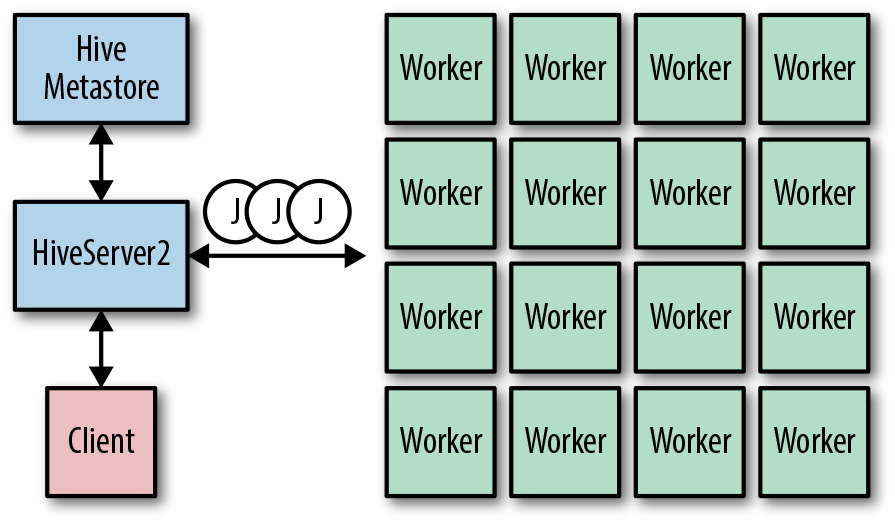
Figure 1-8. High-level overview of Hive operation
Hive is not generally considered to be an interactive query engine (although recently speed improvements have been made via long-lived processes which begin to move it into this realm). Many queries result in chains of MapReduce jobs that can take many minutes (or even hours) to complete. Hive is thus ideally suited to offline batch jobs for extract, transform, load (ETL) operations; reporting; or other bulk data manipulations. Hive-based workflows are a trusted staple of big data clusters and are generally extremely robust. Although Spark SQL is increasingly coming into favor, Hive remains—and will continue to be—an essential tool in the big data toolkit.
We will encounter Hive again when discussing how to deploy it for high availability in Chapter 12.
Going deeper
Much information about Hive is contained in blog posts and other articles spread around the web, but there are some good references:
-
The Apache Hive wiki (contains a lot of useful information, including the HQL language reference)
-
Programming Hive, by Dean Wampler, Jason Rutherglen, and Edward Capriolo (O’Reilly)
Note
Although we covered it in “Computational Frameworks”, Spark is also a key player in the analytical SQL space. The Spark SQL functionality supports a wide range of workloads for both ETL and reporting and can also play a role in interactive query use cases. For new implementations of batch SQL workloads, Spark should probably be considered as the default starting point.
Apache Impala
Apache Impala is a massively parallel processing (MPP) engine designed to support fast, interactive SQL queries on massive datasets in Hadoop or cloud storage. Its key design goal is to enable multiple concurrent, ad hoc, reporting-style queries covering terabytes of data to complete within a few seconds. It is squarely aimed at supporting analysts who wish to execute their own SQL queries, directly or via UI-driven business intelligence (BI) tools.
In contrast to Hive or Spark SQL, Impala does not convert queries into batch jobs to run under YARN. Instead it is a standalone service, implemented in C++, with its own worker processes which run queries, the Impala daemons. Unlike with Hive, there is no centralized query server; each Impala daemon can accept user queries and acts as the coordinator node for the query. Users can submit queries via JDBC or ODBC, via a UI such as Hue, or via the supplied command-line shell. Submitted queries are compiled into a distributed query plan. This plan is an operator tree divided into fragments. Each fragment is a group of plan nodes in the tree which can run together. The daemon sends different instances of the plan fragments to daemons in the cluster to execute against their local data, where they are run in one or more threads within the daemon process.
Because of its focus on speed and efficiency, Impala uses a different execution model, in which data is streamed from its source through a tree of distributed operators. Rows read by scan nodes are processed by fragment instances and streamed to other instances, which may be responsible for joining, grouping, or aggregation via exchange operators. The final results from distributed fragment instances are streamed back to the coordinator daemon, which executes any final aggregations before informing the user there are results to fetch.
The query process is outlined in Figure 1-9. A client chooses an Impala daemon server to which to submit its query. This coordinator node compiles and optimizes the query into remote execution fragments which are sent to the other daemons in the cluster (query initialization). The daemons execute the operators in the fragments and exchange rows between each other as required (distributed execution). As they become available, they stream the results to the coordinator, which may perform final aggregations and computations before streaming them to the client.
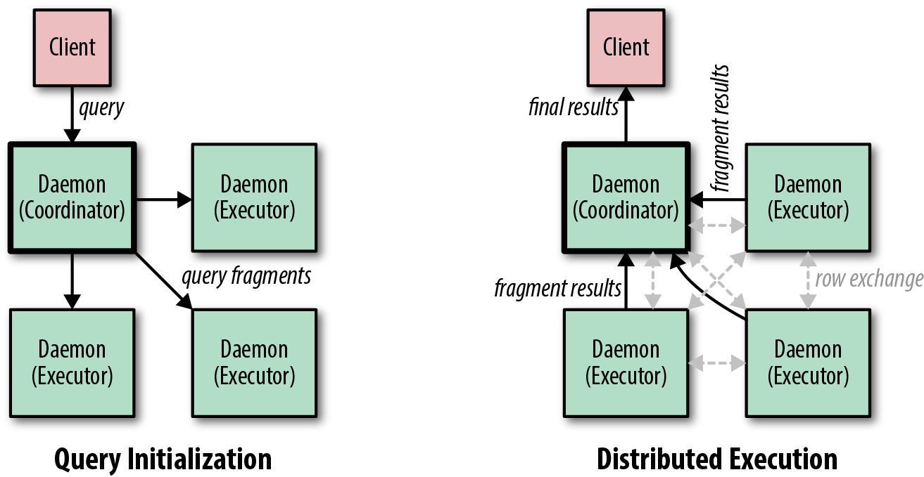
Figure 1-9. A simplified view of the query execution process in Impala
Impala can read data from a wide range of data sources, including text files, HBase tables, and Avro, but its preferred on-disk format is Parquet. Impala can take advantage of the fact that Parquet files store data by columns to limit the data read from disk to only those columns referenced in the query itself. Impala also uses predicate pushdown to filter out rows right at the point that they are read. Currently Impala can read data stored in HDFS, Apache HBase, Apache Kudu, Amazon S3, and Microsoft Azure Data Lake Store (ADLS).
Going deeper
For more details on Impala, we recommend the following sources:
-
Getting Started with Impala, by John Russell (O’Reilly)
Also consider
There are many more analytical frameworks out there. Some other SQL-based distributed query engines to certainly bear in mind and consider for your use cases are:
-
Apache Phoenix (based on Apache HBase, discussed in the next section)
Storage Engines
The original storage engine in the Hadoop ecosystem is HDFS, which excels at storing large amounts of append-only data to be accessed in sequential scans. But what about other access patterns, such as random record retrieval and updates? What about document search? Many workloads deal with large and varied datasets but are not analytical in nature. To cater to these different use cases, a few projects have been developed or adapted for use with Hadoop.
Apache HBase
The desire by some early web companies to store tens of billions to trillions of records and to allow their efficient retrieval and update led to the development of Apache HBase—a semi-structured, random-access key-value store using HDFS as its persistent store. As with many of the Hadoop projects, the original blueprint for the framework came from a paper published by Google describing its system Bigtable. Essentially, HBase provides a means by which a random-access read/write workload (which is very inefficient for HDFS) is converted to sequential I/O (which HDFS excels at).
HBase is not a relational store. Instead, it stores semi-structured key-value pairs, called cells, in a distributed table. HBase subdivides the cell key into a hierarchy of components to allow related cells to be stored and accessed efficiently together. The first portion of the key is called the row key, and it defines a logical grouping of cells, called a row. Next, the key is further subdivided into column families, which again represent a grouping of cells. Column families are stored separately in memory and on disk, and there are usually no more than a handful per table. Column families are the only part of the key schema that need to be defined when the table is created. Within a column family there is a further subdivision, called a column qualifier, of which there can be millions or more per row. Finally, each cell has a timestamp which defines a version. Multiple cells with different timestamps but otherwise the same key can be stored as different versions. HBase treats each component of the key (apart from the timestamp) and the value as arrays of bytes. As a result, HBase doesn’t impose any restrictions on, or have any knowledge of, types in any part of the cell, making it a semi-structured store.
In HBase, cells are stored in order according to their key components. They are sorted first by their row key and then by column family, column qualifier, and finally by timestamp. HBase employs horizontal partitioning—that is, the cells in a table are divided up into partitions, which are distributed around the cluster. The space of row keys in a table is divided up into partitions called regions, each responsible for a nonoverlapping range of the sorted row keys. The boundaries between regions are called region splits. For example, if you know your rows will have row keys with a random alphabetical prefix, you might create your table initially with 26 regions with splits at b, c, d, ..., v, w, x, y, z. Any key starting with a will go in the first region, with c the third region and z the last region. New splits can be added manually or can be automatically created by HBase for busy regions. In this way, a table can be easily distributed and scaled.
The learning curve for operational aspects of HBase can be steep, and it is not necessarily for the faint of heart. Getting the right design for the table and the cell keys is absolutely critical for the performance of your given use case and access pattern. Designing the right table layout requires a solid working understanding of how HBase works, or you are liable to end up with pathological behaviors, such as full-table scans, region hotspotting, or compaction storms. HBase excels at servicing random I/O workloads: well-distributed write or read requests for relatively small groups of cells, via either row gets or range scans. It is not as good at supporting much larger scans, such as those that are typical in analytical workloads. These are expensive to execute and return to the client. Such workloads are typically much better performed directly against the HDFS files themselves.
If managed well and used correctly, HBase is one of the most valuable tools in the ecosystem and can deliver blazing fast performance on huge datasets. It should absolutely be used—just be sure you are using it for the right thing and in the right way.
Going deeper
There are some absolute must-read references if you are serious about using or running HBase:
-
HBase: The Definitive Guide, 2nd Edition, by Lars George (O’Reilly)
-
Architecting HBase Applications, by Jean-Marc Spaggiari and Kevin O’Dell (O’Reilly)
Apache Kudu
One of the principal pain points of the traditional Hadoop-based architecture is that, in order to support both efficient high-throughput analytics and low-latency random-access reads on the same data, multiple storage engines must be used. This results in relatively complex ingestion and orchestration pipelines. Such use cases require something like HBase or Accumulo to service the random-access queries, along with a combination of HDFS, Parquet and Impala, Spark SQL, or Hive for the analytical workloads.
If the incoming data includes updates to existing rows, the picture becomes even more complicated, as it can require wholesale rewrites of data on HDFS or complex queries based on application of the latest deltas. Recognizing this, the creators of Kudu set out to create a storage and query engine that could satisfy both access patterns (random-access and sequential scans) and efficiently allow updates to existing data. Naturally, to allow this, some performance trade-offs are inevitable, but the aim is to get close to the performance levels of each of the native technologies—that is, to service random-access reads within tens of milliseconds and perform file scans at hundreds of MiB/s.
Kudu is a structured data store which stores rows with typed columns in tables with a predefined schema. A subset of the columns is designated as the primary key for the table and forms an index into the table by which Kudu can perform row lookups. Kudu supports the following write operations: insert, update, upsert (insert if the row doesn’t exist, or update if it does), and delete. On the read side, clients can construct a scan with column projections and filter rows by predicates based on column values.
Kudu distributes tables across the cluster through horizontal partitioning. A table is broken up into tablets through one of two partitioning mechanisms, or a combination of both. A row can be in only one tablet, and within each tablet, Kudu maintains a sorted index of the primary key columns. The first partitioning mechanism is range partitioning and should be familiar to users of HBase and Accumulo. Each tablet has an upper and lower bound within the range, and all rows with partition keys that sort within the range belong to the tablet.
The second partitioning mechanism is hash partitioning. Users can specify a fixed number of hash buckets by which the table will be partitioned and can choose one or more columns from the row that will be used to compute the hash for each row. For each row, Kudu computes the hash of the columns modulo the number of buckets and assigns the row to a tablet accordingly.
The two partitioning mechanisms can be combined to provide multiple levels of partitioning, with zero or more hash partitioning levels (each hashing a different set of columns) and a final optional range partition. Multilevel partitioning is extremely useful for certain use cases which would otherwise be subject to write hotspotting. For example, time series always write to the end of a range, which will be just one tablet if only range partitioning is used. By adding a hash partition on a sensible column, the writes can be spread evenly across all tablets in the table and the table can be scaled by dividing each hash bucket up by range.
With all storage and query engines, choosing the right schema and table layout is important for efficient operation. Kudu is no different, and practitioners will need to familiarize themselves with the trade-offs inherent in different row schemas and partitioning strategies in order to choose the optimal combination for the use case at hand. Common use cases for Kudu include:
-
Large metric time series, such as those seen in IoT datasets
-
Reporting workloads on large-scale mutable datasets, such as OLAP-style analyses against star schema tables
Going deeper
The best place to start to learn more about Kudu is the official project documentation. Other resources well worth reading include:
-
“Kudu: Storage for Fast Analytics on Fast Data”, by Todd Lipcon et al. (the original paper outlining the design and operation of Kudu)
-
Getting Started with Kudu, by Jean-Marc Spaggiari et al. (O’Reilly)
Apache Solr
Sometimes SQL is not enough. Some applications need the ability to perform more flexible searches on unstructured or semi-structured data. Many use cases, such as log search, document vaults, and cybersecurity analysis, can involve retrieving data via free-text search, fuzzy search, faceted search, phoneme matching, synonym matching, geospatial search, and more. For these requirements, often termed enterprise search, we need the ability to automatically process, analyze, index, and query billions of documents and hundreds of terabytes of data. There are two primary technologies in the ecosystem at present: Apache Solr and Elasticsearch. We cover only Apache Solr here, but Elasticsearch is also a great choice for production deployments. Both are worth investigating carefully for your enterprise search use case.
To support its search capabilities, Solr uses inverted indexes supplied by Apache Lucene, which are simply maps of terms to a list of matching documents. Terms can be words, stems, ranges, numbers, coordinates, and more. Documents contain fields, which define the type of terms found in them. Fields may be split into individual tokens and indexed separately. The fields a document contains are defined in a schema.
The indexing processing and storage structure allows for quick ranked document retrieval, and a number of advanced query parsers can perform exact matching, fuzzy matching, regular expression matching, and more. For a given query, an index searcher retrieves documents that match the query’s predicates. The documents are scored and, optionally, sorted according to certain criteria; by default, the documents with the highest score are returned first.
In essence, Solr wraps the Lucene library in a RESTful service, which provides index management and flexible and composable query and indexing pipelines. Through the SolrCloud functionality, a logical index can be distributed across many machines for scalable query processing and indexing. Solr can additionally store its index files on HDFS for resilience and scalable storage.
Solr stores documents in collections. Collections can be created with a predefined schema, in which fields and their types are fixed by the user. For use cases that deal with documents with arbitrary names, dynamic fields can be used. These specify which type to use for document fields that match a certain naming pattern. Solr collections can also operate in so-called schemaless mode. In this mode, Solr guesses the types of the supplied fields and adds new ones as they appear in documents.
SolrCloud allows collections to be partitioned and distributed across Solr servers and thus to store billions of documents and to support high query concurrency. As with all storage and query engines, Solr has its strengths and weaknesses. In general, a well-operated and configured SolrCloud deployment can support distributed collections containing billions of documents, but you must take care to distribute query and indexing load properly. The strengths of Solr lie in its flexible querying syntax and ability to do complex subsecond searches across millions of documents, ultimately returning tens to hundreds of documents to the client. It is generally not suitable for large-scale analytical use cases which return millions of documents at a time. And for those who can’t live without it, Solr now supports a SQL dialect for querying collections.
You’ll learn more about using Solr in highly available contexts in “Solr”.
Going deeper
We have only covered the very basics of Solr here. We highly recommend that you consult the official documentation, which has much more detail about schema design and SolrCloud operation. The following are also worth a look:
-
Solr in Action, 3rd Edition, by Trey Grainger and Timothy Potter (Manning). Although slightly dated, this resource contains an excellent description of the inner workings of Solr.
-
Solr ’n Stuff. Yonik Seeley’s blog contains a wealth of background information about various Solr features and an “Unofficial Solr Guide.”
Also consider
As we noted earlier, Elasticsearch is a strong alternative to Solr.
Apache Kafka
One of the primary drivers behind a cluster is to have a single platform that can store and process data from a multitude of sources. The sources of data within an enterprise are many and varied: web logs, machine logs, business events, transactional data, text documents, images, and more. This data arrives via a multitude of modes, including push-based, pull-based, batches, and streams, and in a wide range of protocols: HTTP, SCP/SFTP, JDBC, AMQP, JMS, and more. Within the platform ecosystem, there are multiple sinks for incoming data: HDFS, HBase, Elasticsearch, and Kudu, to name but a few. Managing and orchestrating the ingestion into the platform in all these modes can quickly become a design and operational nightmare.
For streaming data, in particular, the incumbent message broker technologies struggle to scale to the demands of big data. Particular pain points are the demands of supporting hundreds of clients, all wanting to write and read at high bandwidths and all wanting to maintain their own positions in the streams. Guaranteeing delivery in a scalable way using these technologies is challenging, as is dealing with data backlogs induced by high-volume bursts in incoming streams or failed downstream processes. These demands led directly to the development of Apache Kafka at LinkedIn.
Tip
Read more about the background and motivations for a log-based, publish/subscribe architecture in “The Log: What every software engineer should know about real-time data’s unifying abstraction”.
Apache Kafka is a publish/subscribe system designed to be horizontally scalable in both volume and client read and write bandwidth. Its central idea is to use distributed, sequential logs as the storage mechanism for incoming messages and to allow clients, or groups of clients, to consume data from a given point using simple numerical offsets. Kafka has become a critical glue technology, providing a resilient and highly available ingestion buffer, which integrates multiple upstream sources and downstream sinks. Increasingly, stream processing and stateful querying of streams is supported within the Kafka ecosystem itself, with Kafka operating as the system of record.
The fundamental data structure in Kafka is the topic, which is a sequence of messages (or records) distributed over multiple servers (or brokers). Each topic can be created with multiple partitions, each of which is backed by an on-disk log. For resilience, partitions have multiple replicas residing on different brokers.
Messages in Kafka are key-value pairs, where the key and value are arbitrary byte arrays. Clients publish messages to partitions of Kafka topics via producers. Each partition of a topic is an ordered and immutable log. New messages are appended sequentially to the end of the log, which makes the I/O operation very efficient. Within the partition, each message is written together with an offset, which is an always-increasing index into the log. Clients can read from topics using consumers. For scalability, separate consumers can be combined into a consumer group. Consumers can retrieve their last known offset on startup and easily resume where they left off.
Kafka can be used in many ways. Most commonly, it is used as a scalable buffer for data streaming to and from storage engines on Hadoop. It is also frequently used as a data interchange bus in flexible stream processing chains, where systems such as Kafka Connect, Apache Flume, or Spark Streaming consume and process data and write their results out to new topics.
Increasingly, architectures are being built in which Kafka acts as the central system of record and temporary views are built in external serving systems, like databases and key-value stores. It is for this reason that we categorized Kafka as a storage engine rather than as an ingestion technology. However it is used, Kafka is a key integration technology in enterprise big data platforms.
Going deeper
There is a wealth of information about Kafka’s background and usage. Some good places to start include:
-
Kafka: The Definitive Guide, by Gwen Shapira, Neha Narkhede, and Todd Palino (O’Reilly)
-
I Heart Logs, by Jay Kreps (O’Reilly)
Ingestion
There are a lot of technologies in the ingestion space—too many to cover in this survey. Traditionally, two of the main ingestion technologies have been Apache Flume, which is targeted at scalable ingestion for streams of data, and Apache Sqoop, which is focused on importing and exporting data in relational databases. Many other options have emerged, though, to simplify the process of ingestion pipelines and to remove the need for custom coding.
Two notable open source options are:
Orchestration
Batch ingestion and analytics pipelines often consist of multiple dependent phases, potentially using different technologies in each phase. We need to orchestrate and schedule such pipelines and to be able to express their complex interdependencies.
Apache Oozie
Apache Oozie is the job scheduling and execution framework for Hadoop. The basic units of execution within Oozie jobs are actions, which represent tasks that run in the Hadoop ecosystem, such as Hive queries or MapReduce jobs. Actions are composed into workflows, which represent logical sequences or orderings of tasks that need to be run together. Workflows can be run to a schedule via coordinators, which in turn can be grouped together into bundles for logical grouping of applications. An Oozie job can refer to a workflow, coordinator, or bundle.
Oozie jobs are defined via XML files. Each workflow contains a directed (acyclic) graph of actions, basically akin to a flowchart of processing. Coordinators define an execution schedule for workflows, based on time intervals and input dataset availability. Bundles define groups of related coordinators with an overall kickoff time.
Jobs are submitted to the Oozie server, which validates the supplied XML and takes care of the job life cycle. This means different things for different job types. For workflows, it means starting and keeping track of individual action executions on the Hadoop cluster and proceeding through the graph of actions until the workflow completes successfully or encounters an error. For coordinators, the Oozie server arranges for workflows to be started according to the schedule and checks that all input datasets are available for the particular instance of the workflow execution, potentially holding it back until its input data is ready. The Oozie server runs each of the coordinators defined in a bundle.
Workflow actions come in two flavors: asynchronous and synchronous. The majority of actions are run asynchronously on YARN via launchers. Launchers are map-only jobs which, in turn, may submit a further Hadoop job (e.g., Spark, MapReduce, or Hive). This architecture allows the Oozie server to remain lightweight and, consequently, to easily run hundreds of actions concurrently. It also insulates long-running applications from Oozie server failures; because the job state is persisted in an underlying database, the Oozie server can pick up where it left off after a restart without affecting running actions. Some actions are considered lightweight enough to not need to be run via YARN but instead run synchronously, directly in the Oozie server. These include sending emails and some HDFS commands. Oozie job definitions and all associated files and libraries must be stored in HDFS, typically in a directory per application. Oozie exposes a RESTful HTTP API backed by a multithreaded web server through which a user submits, monitors, and controls jobs.
We cover Oozie further in relation to high availability in “Oozie”.
Also consider
Oozie isn’t everyone’s cup of tea, and a couple of very capable contenders have emerged. They are arguably more flexible and usable and well worth considering for greenfield deployments:
Summary
We have covered a fair amount of ground in this primer, beginning with the basic definition of a cluster, which we will cover more in the next chapter. From there, we looked at the core components of Hadoop clusters, computational frameworks, SQL analytics frameworks, storage engines, ingestion technologies, and finally, orchestration systems. Table 1-2 briefly summarizes the components that were covered and outlines their primary intended functionality.
| Project | Description | Used for | Depends on |
|---|---|---|---|
ZooKeeper |
Distributed configuration service |
Sharing metadata between distributed processes and distributed locking |
- |
HDFS |
Distributed file storage |
Scalable bulk storage of immutable data |
ZooKeeper |
YARN |
Distributed resource scheduling and execution framework |
Frameworks requiring scalable, distributed compute resources |
ZooKeeper, HDFS |
MapReduce |
Generic distributed computation framework |
Batch compute workloads |
YARN, HDFS |
Spark |
Generic distributed computation framework |
Batch, analytical SQL, and streaming workloads |
Resource scheduler (e.g., YARN or Mesos), data sources (e.g., HDFS, Kudu) |
Hive |
SQL analytics query framework |
Analytical SQL workloads |
YARN, data sources (e.g., HDFS, Kudu) |
Impala |
MPP SQL analytics engine |
Analytical, interactive SQL workloads |
Data sources (HDFS, Kudu, HBase) |
HBase |
Distributed, sorted store for hierarchical key-value data |
Random, low-latency read/write access to row-based data with structured keys |
HDFS, ZooKeeper |
Kudu |
Distributed store for structured data |
Combined random read/write access and analytical workloads |
- |
Solr |
Enterprise search framework |
Scalable document indexing and querying on arbitrary fields |
HDFS, ZooKeeper |
Kafka |
Distributed pub/sub messaging framework |
Scalable publishing and consumption of streaming data |
ZooKeeper |
Oozie |
Workflow scheduler |
Regular and on-demand data processing pipelines |
- |
With this working knowledge under your belt, the rest of the book should be easier to digest. If you forget some of the details, you can always use this section to refamiliarize yourself with the key technologies.
1 In common with most open source projects, we avoid the term slave wherever possible.
Get Architecting Modern Data Platforms now with the O’Reilly learning platform.
O’Reilly members experience books, live events, courses curated by job role, and more from O’Reilly and nearly 200 top publishers.

