Chapter 4. Building Causal Diagrams from Scratch
At this point, you may be wondering where the [causal diagram] comes from. It’s an excellent question. It may be the question. A [CD] is supposed to be a theoretical representation of the state-of-the-art knowledge about the phenomena you’re studying. It’s what an expert would say is the thing itself, and that expertise comes from a variety of sources. Examples include economic theory, other scientific models, conversations with experts, your own observations and experiences, literature reviews, as well as your own intuition and hypotheses.
Our goal in this book is always to measure the impact of one variable on another, which we can represent as a “starter” CD (Figure 4-1).
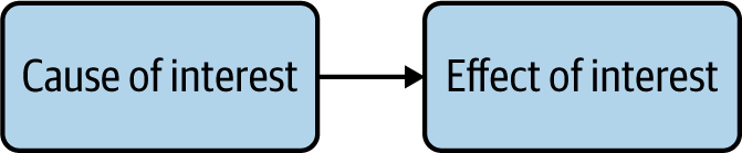
Figure 4-1. The simplest possible CD
Once you have drawn that relationship, what comes next? How can you know what other variables you should include or not? Many authors say you should rely on expert knowledge, which is fine if you work in an established field like economics or epidemiology. But my perspective in this book is that you’re likely “behavioral scientist number one” in your organization and therefore you need to be able to start from a blank slate.
In this chapter, I’ll outline a recipe to get you from the basic CD in Figure 4-1 to a workable CD. As we go through the process, please keep in mind our ultimate goal of understanding what drives behaviors so that we can draw relevant and actionable conclusions for our business. Our objective is not to build a complete and precise knowledge of the whole world. Shortcuts and approximations are fair game, and everything should be assessed according to a single criterion: is this helping me with my business goal?
In addition, the recipe I’ll outline is not a mechanical algorithm that you could follow blindly to get to the right CD. On the contrary, business sense, common sense, and data insights will be crucial. We’ll go back and forth between our qualitative understanding of the causal situation at hand and the quantitative relationships present in the data, cross-checking one with the other until we feel that we have a satisfactory result. “Satisfactory” is an important word here: in applied settings, you usually can’t tell your manager that you’ll give them the right answer in three years. You need to give them the least bad answer possible in the short term, while planning the data collection work that will improve your answer over the years.
In the next section, I’ll present the business problem for this chapter and the corresponding variables of interest. We’ll then progressively build out the corresponding CD along the following recipe, with one section per step:
-
Identify variables that could/should potentially be included in the CD.
-
Determine if the variables should be included.
-
Iterate the process as needed.
-
Simplify the diagram.
Let’s get started!
Business Problem and Data Setup
For this section, we’ll be working with a real-world data set of hotel bookings for two hotels located within the same city.1 The data and packages that we’ll use are described in the next subsection, and we’ll then do a deeper dive to understand the relationship of interest.
Data and Packages
The GitHub folder for this chapter contains the CSV file chap4-hotel_booking_case_study.csv with the variable listed in Table 4-1.
| Variable name | Variable description |
|---|---|
| NRDeposit (NRD) | Binary 0/1, whether the reservation had a nonrefundable deposit |
| IsCanceled | Binary 0/1, whether the reservation was canceled or not |
| DistributionChannel | Categorical variable with values “Direct,” “Corporate,” “TA/TO” (travel agent/travel organization), “Other” |
| CustomerType | Categorical variable with values “Transient,” “Transient-Party,” “Contract,” “Group” |
| MarketSegment | Categorical variable with values “Direct,” “Corporate,” “Online TA,” “Offline TA/TO,” “Groups,” “Other” |
| Children | Integer, number of children in the reservation |
| ADR | Numeric, average daily rate, total reservation amount/number of days |
| PreviousCancellation | Binary 0/1, whether the customer previously canceled a reservation or not |
| IsRepeatedGuest | Binary 0/1, whether the customer has previously made a reservation at the hotel |
| Country | Categorical, country of origin of the customer |
| Quarter | Categorical, quarter of year for the reservation |
| Year | Integer, year of the reservation |
In this chapter, we’ll use the following packages in addition to the standard ones called out in the preface:
## Rlibrary(rcompanion)# For Cramer V correlation coefficient functionlibrary(car)# For VIF diagnostic function
## Pythonfrommathimportsqrt# For Cramer V calculationfromscipy.statsimportchi2_contingency# For Cramer V calculation
Understanding the Relationship of Interest
We’ll try to answer the question, “Does the type of deposit impact the cancellation rate of bookings?” as expressed in Figure 4-2.
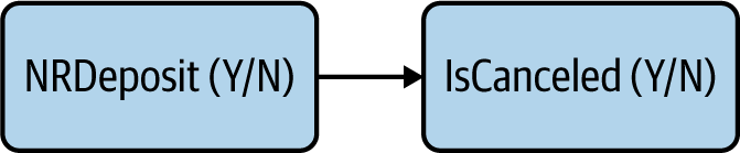
Figure 4-2. Causal relationship of interest
Let’s start by looking at the base cancellation rate by deposit type (I like to look at both the absolute numbers and the percentages, in case some categories have very small numbers):
## R (output not shown)with(dat,table(NRDeposit,IsCanceled))with(dat,prop.table(table(NRDeposit,IsCanceled),1))
## Pythontable_cnt=dat_df.groupby(['NRDeposit','IsCanceled']).\agg(cnt=('Country',lambdax:len(x)))(table_cnt)table_pct=table_cnt.groupby(level=0).apply(lambdax:100*x/float(x.sum()))(table_pct)cntNRDepositIsCanceled006331612304210551982cntNRDepositIsCanceled0073.318048126.681952105.303761194.696239
We can see that the overwhelming majority of bookings have no deposit, with a cancellation rate of about 27%. On the other hand, bookings with nonrefundable deposits (NRDeposit) have a very high cancellation rate. On the face of it, this correlation is surprising. Would changing our policy to “no deposit” for everyone reduce cancellation rates? Behavioral common sense tells us that more likely, the hotels are requesting nonrefundable deposits for “high risk” bookings and there is a confounder, as represented in Figure 4-3.
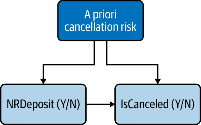
Figure 4-3. The causal relationship is likely confounded
We went pretty quickly from Figure 4-2 to Figure 4-3, but it was an important step: the CD in Figure 4-2 represents a basic business analytics question, “What is the causal relationship between deposit type and cancellation rate?” On the other hand, the CD in Figure 4-3 represents a more informed behavioral hypothesis: “A nonrefundable deposit seems to increase cancellation rate, but that relationship is probably confounded by factors we’ll need to determine.”
A nice aspect of using CDs for behavioral data analysis is that they are a great collaboration tool. Anyone in your organization with minimal knowledge of CDs can look at Figure 4-3 and say, “Well yeah, we require nonrefundable deposits for holiday bookings and these often get canceled because of weather,” or any other tidbit of behavioral knowledge that you couldn’t get otherwise.
At this point, the best next step would be a randomized experiment: assign refundable or nonrefundable deposits to a random sample of customers and you’ll be able to confirm or disprove your behavioral hypothesis. However, you may not be able to do so, or not yet. In the meantime, we’ll try to deconfound the relationship by identifying relevant variables to include.
Identify Candidate Variables to Include
When trying to identify potential variables to include, a natural inclination is to start with the data you have available. This inclination is misleading, akin to the drunk person who looks for their house keys not where they lost them, but under a streetlamp because there is more light there. By doing so, you may be ignoring the most important variables simply because they’re not under your nose. You’re also more likely to take the variables in your data at face value, and not question whether they are the best representation of what’s happening in the real world.
For instance, categorical variables in your data are likely to represent a business-centric perspective rather than a customer-centric perspective, and it may be more appropriate to aggregate some categories together, or even to merge different variables into new ones. In our case, we have a variable MarketSegment and one for the number of children in the reservation. We can confirm by looking at the data that very few corporate customers bring children with them. Therefore we could consider creating a new categorical variable with categories “corporate without children,” “noncorporate without children,” and “noncorporate with children,” setting aside the corporate customers with children as outliers worthy of a separate investigation (maybe the seed for tailored services?).
Instead of falling for this “What You See Is All There Is” bias,2 we’ll start with the behavioral categories outlined in Chapter 2, from the action backward:
-
Actions
-
Intentions
-
Cognition and emotions
-
Personal characteristics
-
Business behaviors
Finally, variables in each one of these categories may be affected by time trends such as linear trends or seasonality, so we’ll add these by default at the end of this section. In order to reinforce the focus on qualitative intuitions, we won’t look at any data until the next section, about validating relationships. Replacing our a priori cancellation risk (as well as other potential confounders) by these categories, our CD now looks like Figure 4-4, with a bunch of unobserved variables added to our two variables of interest.
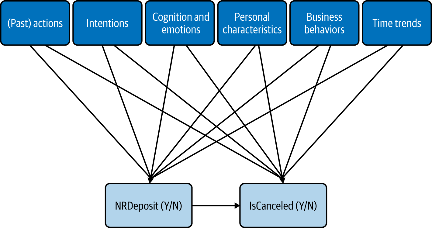
Figure 4-4. Updated CD with categories of potential variables to include
For each of these categories, we’ll now look for variables that may be a cause of either of our two variables of interest.
Actions
When looking for variables to include in the actions category, we’re usually trying to identify past behaviors from the customer that may affect whether the hotel required a nonrefundable deposit (NRD).
An obvious candidate in this case is whether the customer previously canceled. Maybe the hotel is more likely to request an NRD from customers who flaked in the past. It is also conceivable that whatever caused them to cancel in the past is also more likely to make them cancel in the future.
More generally, when one of our variables of interest is itself an action, past behavior is often a good predictive variable to include, even just as a proxy for unobserved personal characteristics. We have two variables related to past behavior in our data: PreviousCancellation and IsRepeatedGuest. Figure 4-5 shows our updated CD, with the unchanged portions in gray.
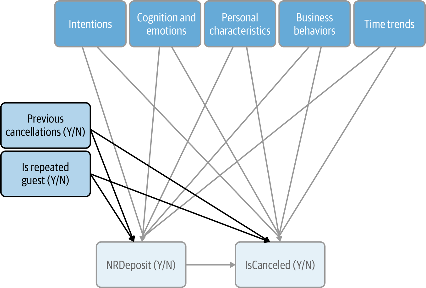
Figure 4-5. Updated CD at the end of the actions step
This is not to say that these are the only relevant past behaviors; they just happen to be the only ones I thought of and that we had data for. Hopefully, you can think of others!
Intentions
Intentions are easy to overlook in data analysis, because they are often missing from our existing data. However, they are one of the most important drivers of behaviors, and they can often be revealed by interviewing customers and employees. They thus represent one of the best illustrations of the benefits of not just looking at existing, available data, but adopting a “behaviors first” approach.
In this case, there are two intentions I can think of: the reason for the trip and the reason for the cancellation (Figure 4-6).
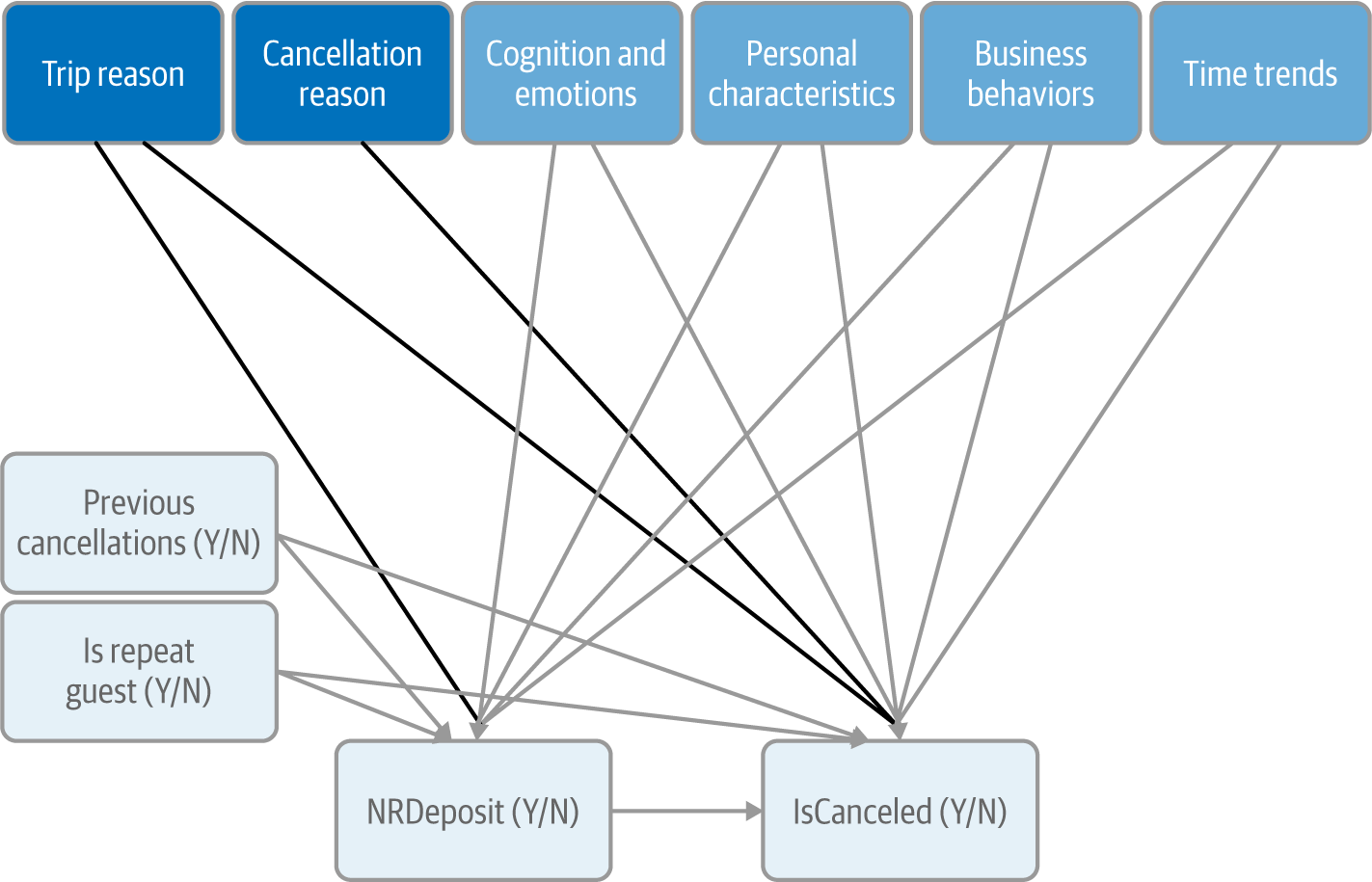
Figure 4-6. Adding intentions to our CD
Note that I represented TripReason as a potential confounder, i.e., with an arrow to both of our variables of interest, whereas CancellationReason affects only IsCanceled. At this point, this is just a behavioral hunch, namely that the reason for the cancellation doesn’t affect the type of deposit. My rationale is that the reason for cancellation is not known at the time of the deposit.
Figure 4-6 also shows the versatility of CDs for behavioral analysis: we can put down these two potential variables in our CD even without knowing the actual list of reasons in either case, which we’ll determine later through interviews. For the time being, we can note that three of the variables available in our data appear to be affected by trip reason and can be included as such: CustomerType, MarketSegment, and DistributionChannel (Figure 4-7). We’ll also revisit these variables in the subsection about personal characteristics.
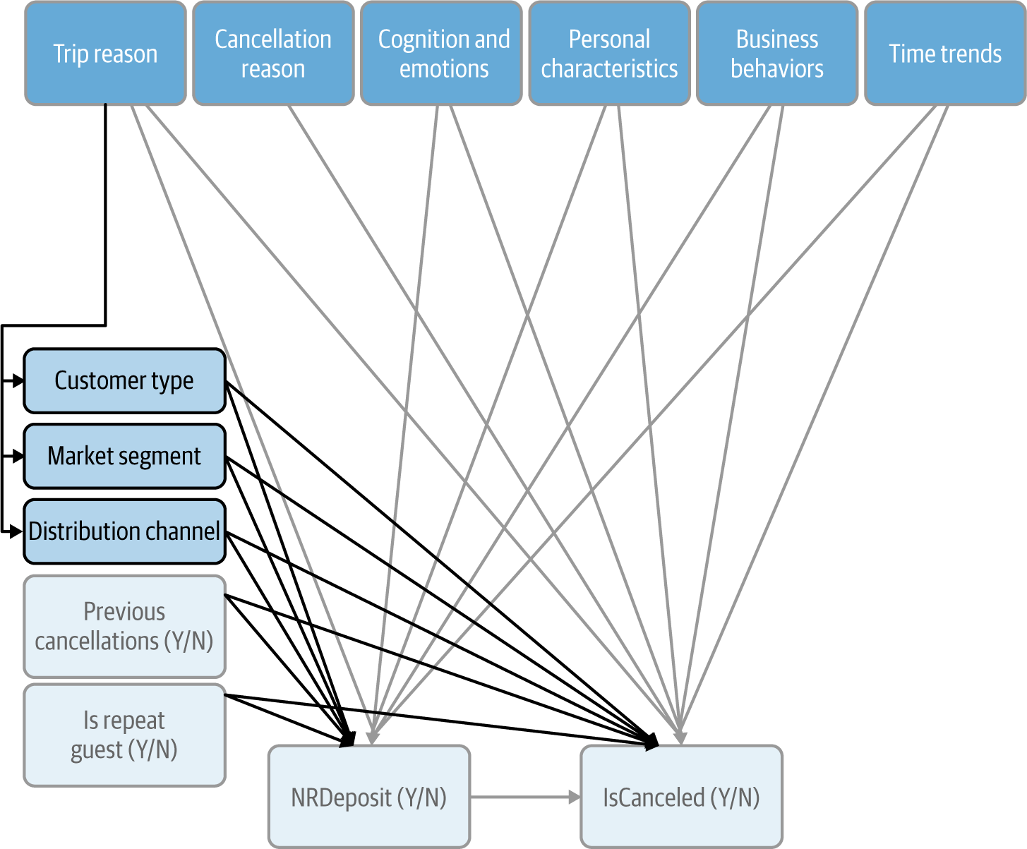
Figure 4-7. Updated CD at the end of the intention step
Cognition and Emotions
When trying to identify relevant social, psychological, or cognitive phenomena for an analysis, I like to zoom in on specific decision points. Here that would be when the customer makes the reservation and when they cancel it.
At the first decision point, customers may not understand that their deposit is nonrefundable, or they may forget it. At the second decision point, they may treat their deposit as a sunk cost and not make efforts to keep their reservations (Figure 4-8).
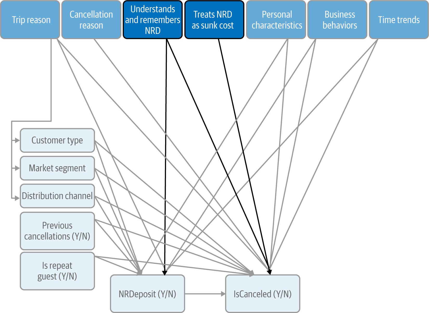
Figure 4-8. Updated CD at the end of the cognition and emotions step
Personal Characteristics
As mentioned in Chapter 2, demographic variables are often valuable not so much for themselves but as proxies for other personal characteristics such as personality traits. The challenge at this step is therefore to resist the pull of whatever demographic variables are present in our data, and stick with our causal-behavioral mindset. A good way to do so is to think about traits first, before looking at demographic variables.
Traits
Based on our knowledge of personality psychology, good candidate traits to cause our cancellation behavior are conscientiousness and neuroticism: it seems plausible that less organized and more carefree people are more likely to end up cancelling a reservation (Figure 4-9).
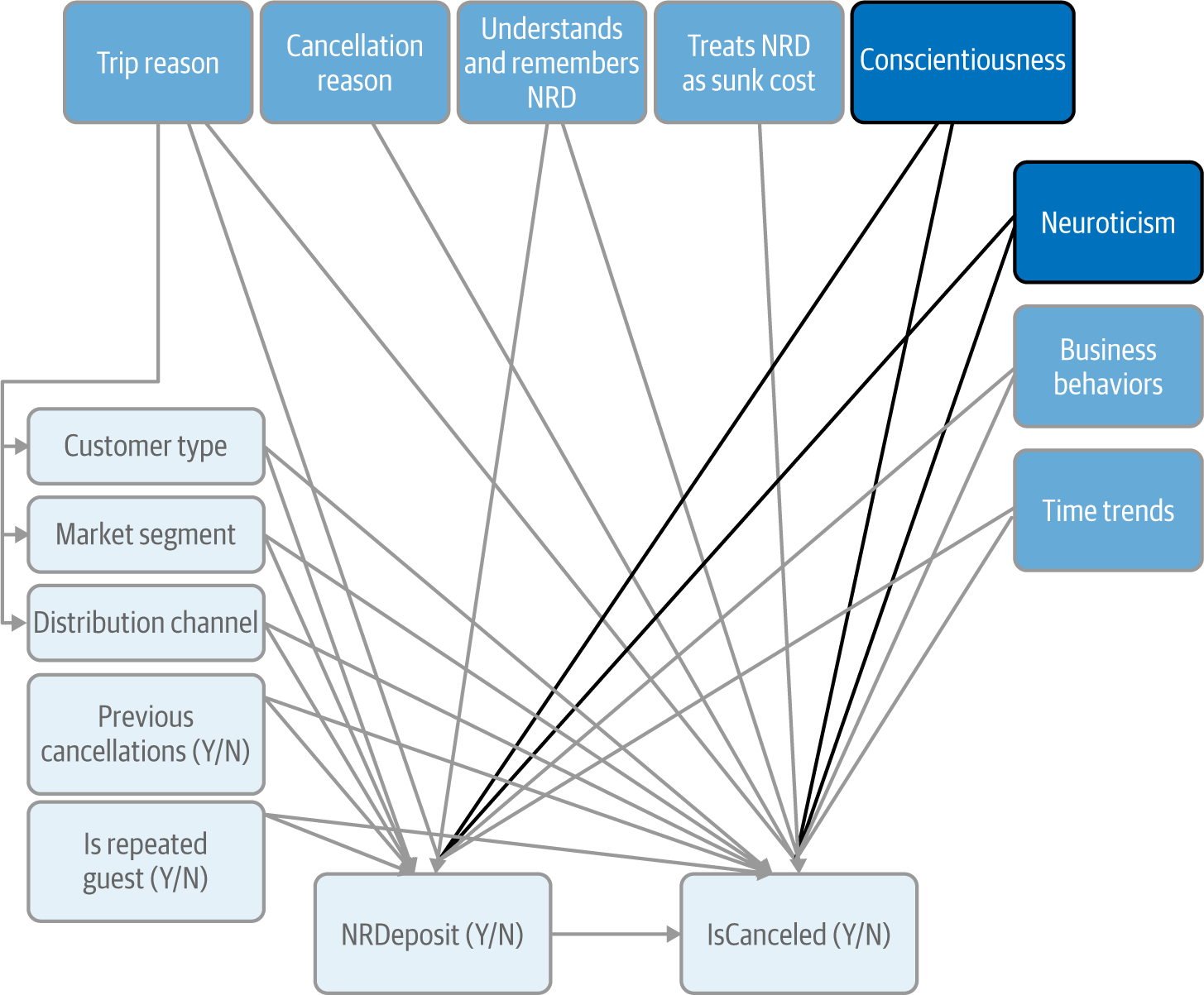
Figure 4-9. CD updated with personality traits
Demographic variables
We noted earlier that we have corporate and noncorporate customers making reservations at the hotels. Beyond the reasons for the trip and for the cancellation, this also affects some other personal characteristics such as price elasticity and income, both of which would affect our two variables of interest. Let’s group these under the heading “financial characteristics.” They are probably somewhat captured by the three variables we saw earlier, CustomerType, MarketSegment, and DistributionChannel, as well as by a few other variables in our data such as Children, ADR (the average daily rate, i.e., the price for a night), and Country (Figure 4-10).
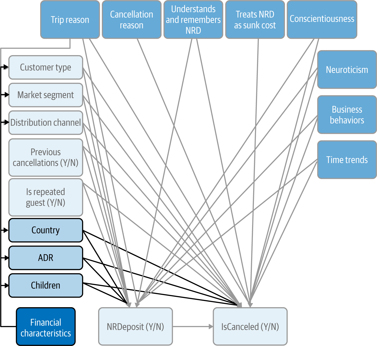
Figure 4-10. CD updated with demographic variables
Business Behaviors
Business behaviors often play a big role in the relationships we’re investigating, but they can easily be overlooked and tricky to integrate.
In this example, business rules obviously play an important role, as they determine which customers will have to provide an NRD. In that sense, they influence all the arrows in the CD going into NRDeposit. We can account for this influence in several ways, depending on the forms it takes.
A business rule may explicitly connect two observable variables (possibly including our variables of interest). Here for instance, we can imagine a business rule stating that all customers who have previously canceled must now provide an NRD. By listing all such rules, we can confirm or disprove all arrows from an observed variable directly into NRDeposit. This may also surface variables that are involved in business rules but are not yet in our data: for example, we could imagine that customers who don’t provide a proof of ID at the time of the reservation must pay an NRD. I said “not yet in our data” because by definition any criterion that is part of a business rule is observable, even if it’s not captured in a database.3
Alternatively, a business rule may be best represented as an additional intermediary variable. For instance, if all reservations during the Christmas holidays must be backed by an NRD, we could create a ChristmasHolidays binary variable with an arrow to NRDeposit. That variable would then mediate the effect of other variables such as CustomerType or Children on NRDeposit.
We don’t know what business rules the two hotels in our example apply so we have to leave that subsection as something that we would want to explore through later interviews.
Time Trends
Finally, there might be some global time trends in our data, such as a progressive increase in the number of reservations requiring an NRD paralleled by a progressive, but unrelated, increase in the cancellation rate. In addition, given how seasonal the hotel industry is, there are probably some cyclical aspects that we would want to capture (Figure 4-11).
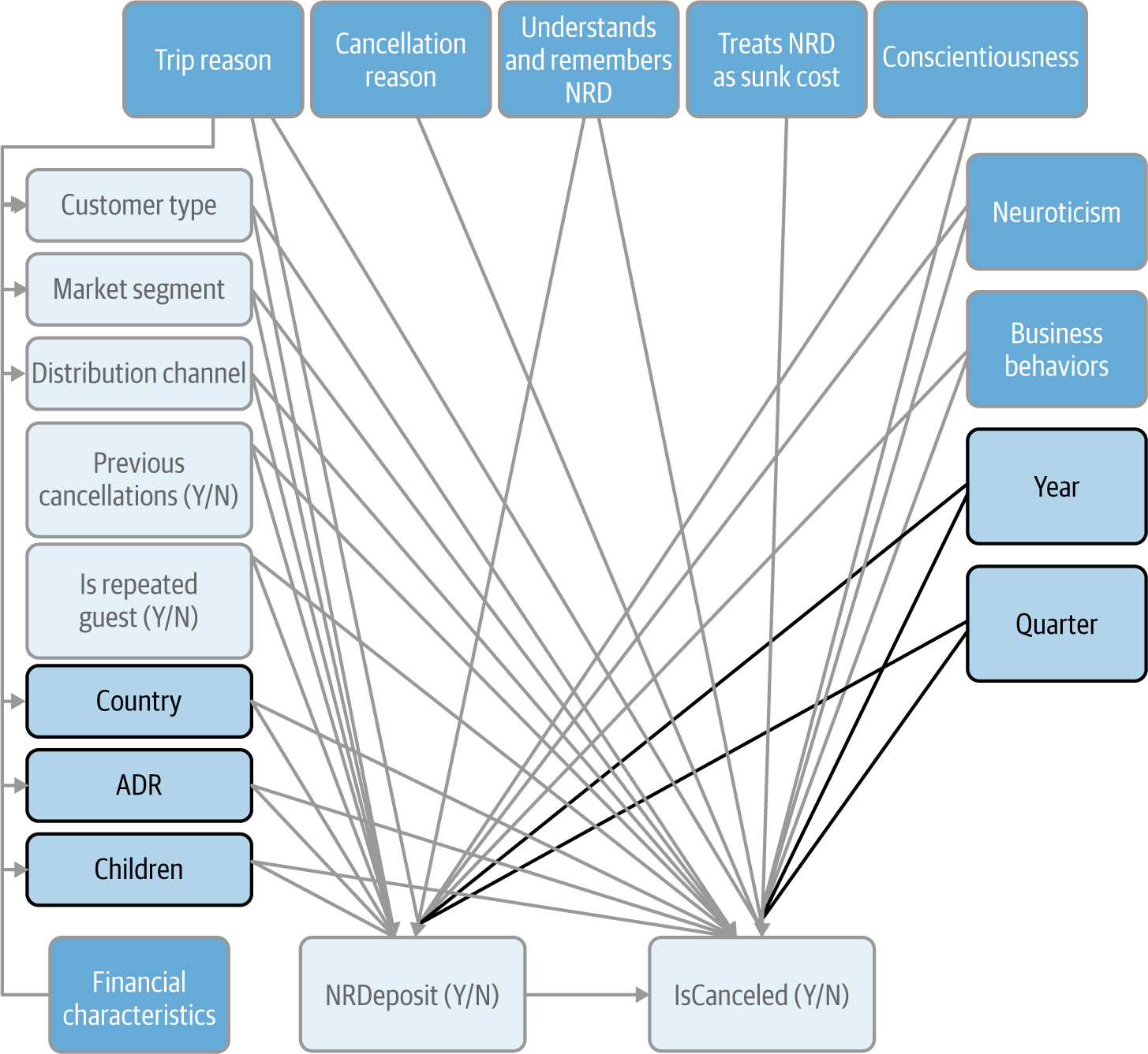
Figure 4-11. Updated CD at the end of the time trends step
Note
In the present case, the Year and Quarter variables only capture trends and cycles. Sometimes it can also make sense to include binary variables to account for specific events that make a certain year stand out or mark a permanent change. An obvious example is COVID-19, which, when the dust settles, will turn out to have been a temporary blip in certain sectors but the beginning of a sea change in others.
With that final addition, Figure 4-11 now has a raft of candidate variables, some observable and some not. In the next section, we’ll see how to confirm which observable variables to keep.
Validate Observable Variables to Include Based on Data
Let’s look at the observable variables we have as candidates at the end of the identification phase (Figure 4-12).
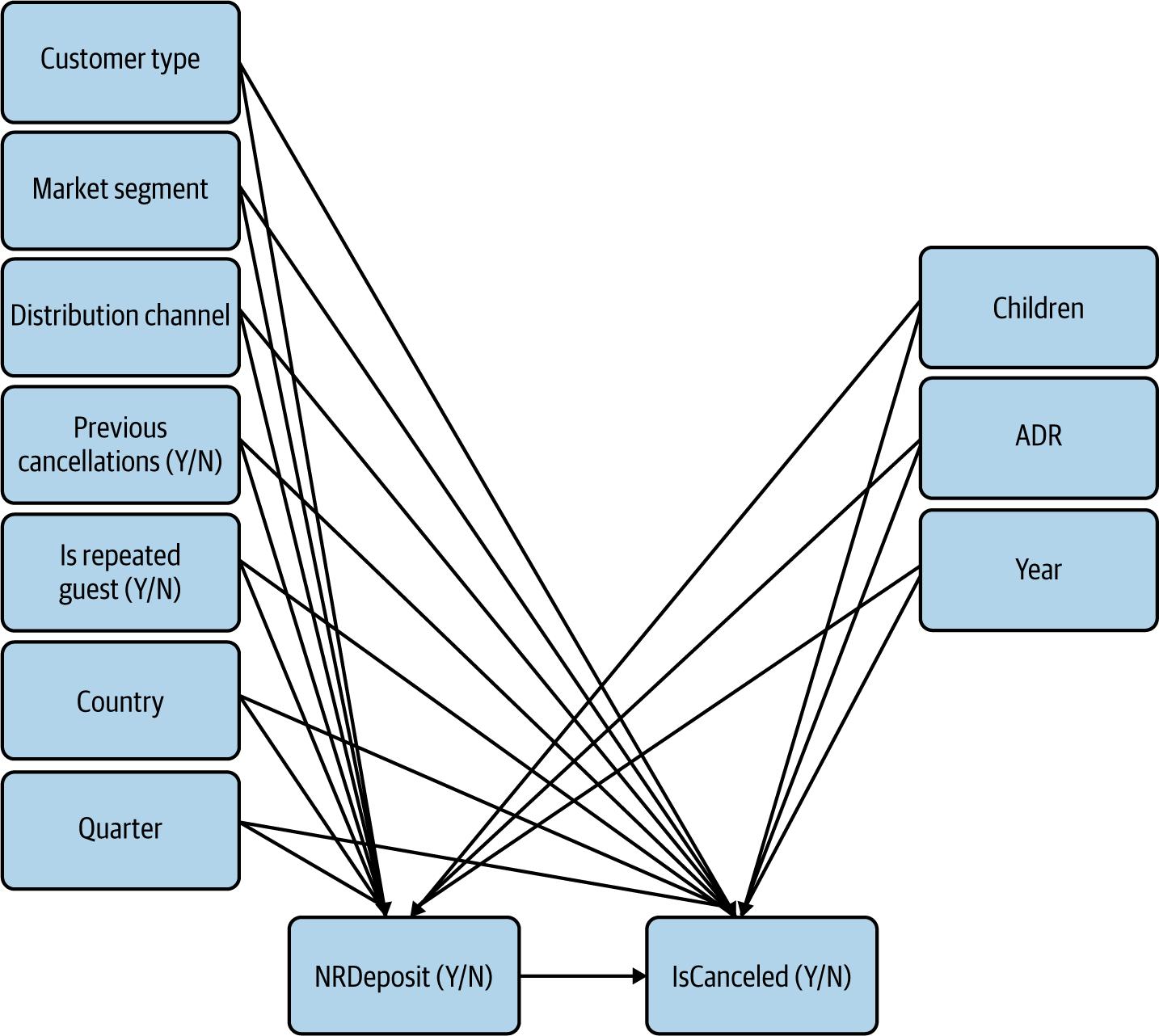
Figure 4-12. Observable variables in our CD, split by categorical (left) and numeric (right)
In this specific example, all of these observable variables are tentatively connected to both of our variables of interest. This is the default situation, but in some cases you may have a very strong a priori rationale to connect a predictor variable to only one of your variables of interest (that was the case, for example, with some of our unobserved variables). When in doubt, I would err on the side of caution and include both connections.
In Figure 4-12, the observable variables are split between categorical (on the left of the CD) and numeric (on the right of the CD). These two types of data call for different quantitative tools, so we’ll see them in turn.
Relationships Between Numeric Variables
Our first step will be to look at the correlation matrix for all the numeric variables in our data. A useful but dirty trick is to convert binary variables to 0/1 (if they’re not already in that format) so that you can treat them as numeric. It allows you to get a sense of the correlation between variables, but don’t tell your statistician friends!
Looking at the rows for your two variables of interest will allow you to see how correlated they are with all the numeric variables in your data set. At a glance, it will also show you any large correlation between these other variables. The strength of the correlation with the cause and effect of interest can then help us determine what to do with a given variable.
How strong is strong? It depends. Remember that our goal is to correctly measure the causal effect of our cause of interest on our effect of interest; as a rule of thumb, you can consider as “strong” any correlation that is of the same order of magnitude (i.e., the same number of zeros between the comma and the first nonzero digit) as the correlation between your cause of interest and your effect of interest.
As you can see in Figure 4-13, the correlation coefficient between our two variables of interest is 0.16. The first column indicates the correlations with NRDeposit and the second column the correlations with IsCanceled. PreviousCancellation has correlation coefficients with our variables of interest that are of the same order of magnitude (0.15 and 0.13, respectively). Similarly, ADR has a correlation coefficient with IsCanceled that is significant by that criterion (0.13).
The “order of magnitude” threshold for inclusion is not scientific in the least, and it can be tightened or loosened depending on how many variables you have at hand. If you have few variables passing the threshold and some other variables are close to it, it is perfectly fine to include them.
You may object that a variable could have a low correlation with either of our variables of interest but still be a confounder that needs to be accounted for. This is true, and you can include a variable even if it is only feebly correlated with our variables of interest, based on a strong theoretical rationale. However, for practical purposes, you should usually focus on variables having at least a moderate level of correlation with our variables of interest.

Figure 4-13. Correlation matrix for numeric and binary variables
If we include all the correlations that are 0.1 or above in absolute value in Figure 4-13 and exclude the others, our CD is now as in Figure 4-14.
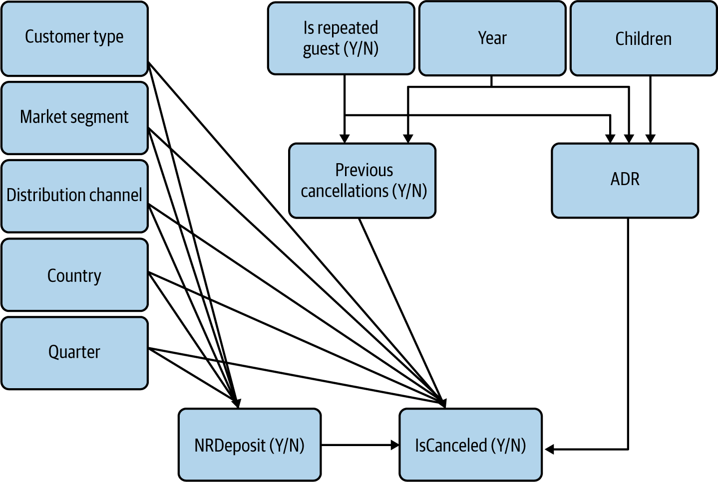
Figure 4-14. CD with updated arrows for the numeric and binary observable variables
While the correlation matrix only gives us symmetrical coefficients that could represent arrows in either direction, I have used some common sense and business knowledge to assume the direction of the arrows. The hotel company has no mastery of time, so we can assume that Years is the cause and not the effect of variables it’s correlated with, although that effect may go through intermediary variables such as trends in society over time. IsRepeatedGuest is a prerequisite for PreviousCancellation; because it refers to a past event, it must also be the cause of ADR or they both share a common cause.
Note
Don’t forget that this is a tentative CD:
-
Some of these correlations are likely false positives (the coefficient appears stronger than it really is, out of sheer randomness) and conversely, some of the smaller correlations may be false negatives.
-
At this stage, we’re tentatively treating correlations as evidence of causation. Some of the arrows we’ve drawn in Figure 4-14 may themselves reflect relationships that are confounded. After adequately measuring the relationship between NRDeposit and IsCanceled, we may want or need to do the same for other relationships (e.g., the one between IsRepeatedGuest and ADR).
Relationships Between Categorical Variables
The same logic applies for categorical variables, with the only complication that we can’t use Pearson’s correlation coefficient. However, a variant of it, Cramer’s V, has been developed for categorical variables. In R, it is implemented in the rcompanion package:
## R>with(dat,rcompanion::cramerV(NRDeposit,IsCanceled))CramerV0.165
You can see that in the case of binary variables, it yields a result that is quite close to the direct application of Pearson’s correlation coefficient. Unfortunately, it is not implemented in Python, but I provide a function to calculate it:
## PythondefCramerV(var1,var2):...returnVV=CramerV(dat_df['NRDeposit'],dat_df['IsCanceled'])(V)0.16483946381640308
Figure 4-15 shows the corresponding correlation matrix, after renaming the variables for readability:
## R
dat <- dat %>%
  rename(CustTyp= CustomerType) %>%
  rename(DistCh = DistributionChannel) %>%
  rename(RepGst = IsRepeatedGuest) %>%
  rename(MktSgmt = MarketSegment) %>%
  rename(IsCanc = IsCanceled) %>%
  rename(PrevCan = PreviousCancellations) %>%
  rename(NRDep = NRDeposit)

## Python
dat_df.rename(columns=
              {"CustomerType": "CustTyp",
               "DistributionChannel": "DistCh",
               "IsRepeatedGuest": "RepGst",
               "MarketSegment": "MktSgmt",
               "IsCanceled": "IsCanc",
               "PreviousCancellations": "PrevCan",
               "NRDeposit": "NRDep"},
              inplace=True)
This correlation yields a variety of insights. Looking at the bottom row, we can see that Quarter is not meaningfully correlated with anything else. This suggests that seasonality is not a relevant factor for our analysis. Conversely, it is possible that a quarter is too coarse a unit of time and that we need to zoom in on very specific time periods such as the Christmas holidays. We can drop Quarter from our CD and replace it with an unobserved variable Seasonality as a cue for future research.
Our three variables for customer segments, CustomerType, MarketSegment, and DistributionChannel, show a mixed pattern, with some very strong and some weak correlations between them. Similarly, their correlations with other variables are all over the place: all three of them have correlations with Country in the 0.1X digits for example, but two of them have high correlations with RepeatedGuest (0.35 and 0.4) whereas the third one has a correlation of only 0.11. This suggests that these variables are not just interchangeable, but that they are capturing some aspects of the same behaviors. This calls for further investigation and most likely creating new variables.
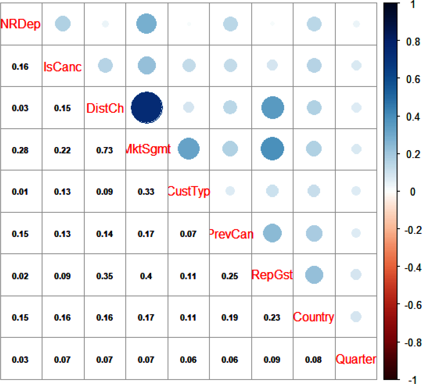
Figure 4-15. Correlation matrix for categorical and binary variables
Applying these insights and the same criterion of including only correlations above 0.1, our CD now looks like Figure 4-16.
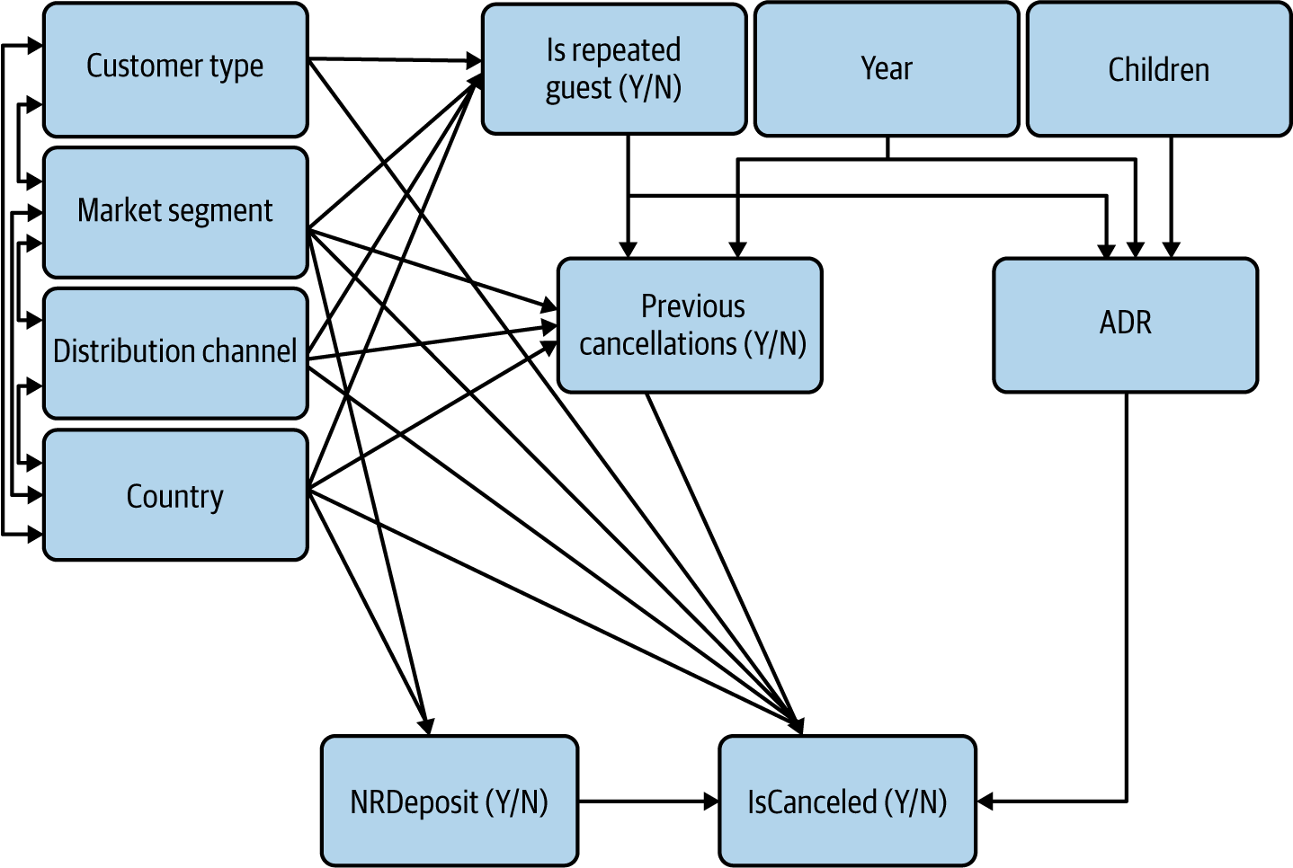
Figure 4-16. CD with updated arrows for the categorical and binary observable variables
Our CD is starting to get moderately complex, but it can for the most part be summarized in a few behavioral arguments:
-
Our four variables on the left reflect personal characteristics and they are significantly correlated with each other. I have chosen to reflect these correlations with double-headed arrows because trying to determine the direction of arrows would be pointless: CustomerType doesn’t cause MarketSegment any more than the other way around. In reality, after doing the necessary interviews, we should create new variables that capture the deeper personal characteristics at play.
-
Personal characteristics appear to affect our variables of interest, potentially causing some confounding.
-
Personal characteristics appear to have affected past behaviors IsRepeatedGuest and PreviousCancellation. (Again, I’m making assumptions on the direction of the effects based on business knowledge. On the face of it, it seems unlikely that having canceled a previous reservation would make someone change country or market segment.) Once we have clarified the nature of the deeper personal characteristics at play, we may decide to fold these past behaviors under some personal characteristics variables, implicitly creating behavioral personas (e.g., “recurring business traveler (Y/N)”).
Relationships Between Numeric and Categorical Variables
Measuring correlations between numeric and categorical variables is a more cumbersome process than measuring correlations within a homogenous category.
Saying that there is a correlation between a numeric and a categorical variable is equivalent to saying that the values of the numeric variable are different on average across the categories of the categorical variable. We can check if this is the case by comparing the mean of the numeric variable across the categories of the categorical variable. For example, we expect that the financial characteristics of the customer may impact the average daily rate for the reservation. It would be best to explore that relationship after having built better variables for customer segmentation, but for the sake of the argument we can use CustomerType:
## R (output not shown)>dat%>%group_by(CustTyp)%>%summarize(ADR=mean(ADR))
## Pythondat_df.groupby('CustTyp').agg(ADR=('ADR',np.mean))Out[10]:ADRCustTypContract92.753036Group84.361949Transient110.062373Transient-Party87.675056
We can see that the average daily rate varies substantially between customer types.
Note
If you’re unsure whether the variations are truly substantial or if they only reflect random sampling errors, you can build confidence intervals for them using the Bootstrap, as explained later in Chapter 7.
In our example, there are two numeric variables whose correlation with categorical variables we may want to check: ADR and Year. We find that ADR varies substantially across customer types but that these are reasonably stable over time, which brings us to our final CD for observable variables (Figure 4-17).
At this point, I’d like to reiterate and expand on my earlier warning: in the process of validating observable variables, I have implicitly assumed that correlation was causation. But maybe these relationships are themselves confounded: the correlation between personal characteristics variables and PreviousCancellation might be entirely caused by the relationship between personal characteristics variables and IsRepeatedGuest.
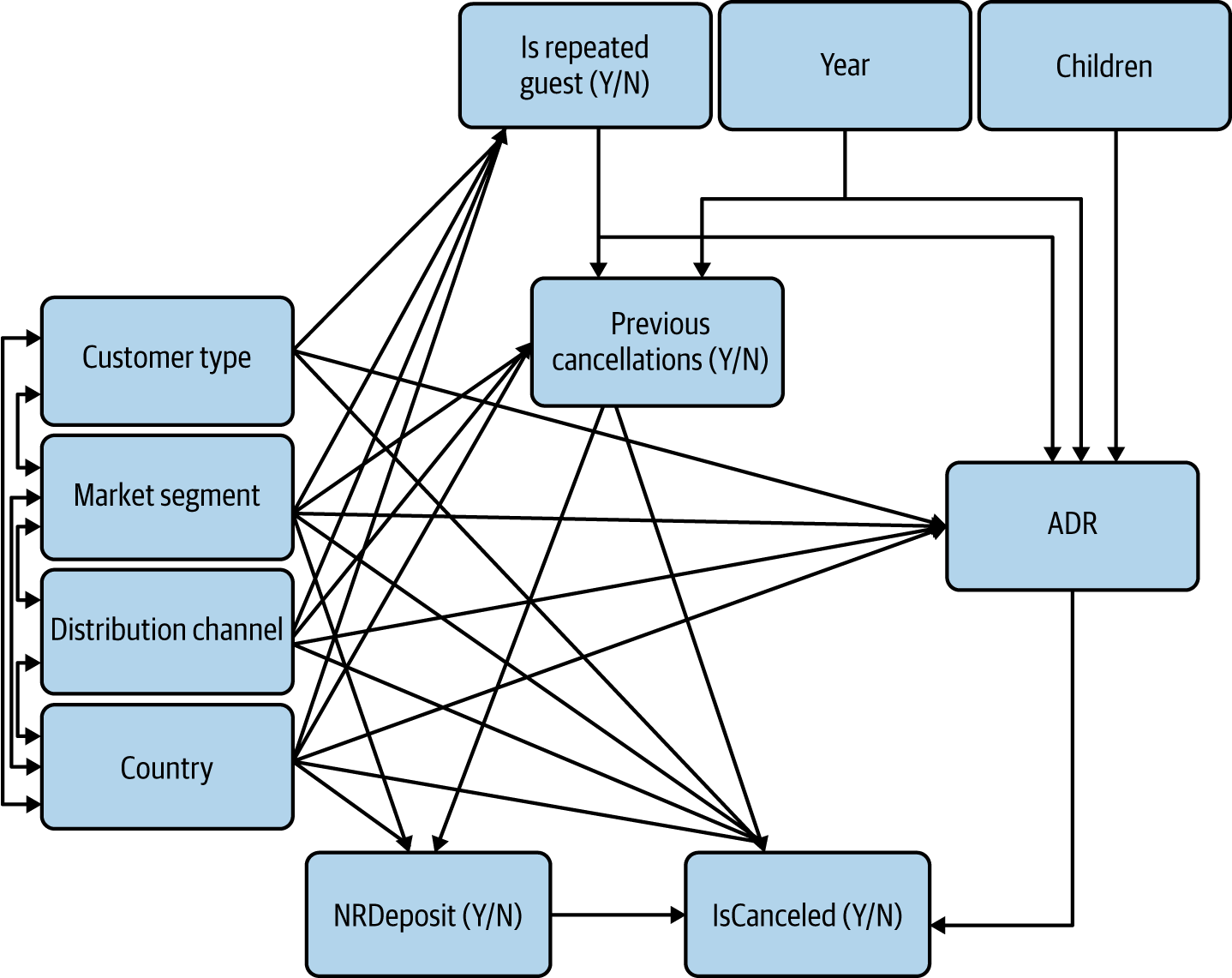
Figure 4-17. Final CD for observable variables
Let’s imagine for instance that business customers are more likely to be repeated guests. They may then also appear to have a higher rate of previous cancellation than leisure customers even though among repeated guests, business and leisure customers have the exact same rate of previous cancellations.
You can think of these causality assumptions as white lies: they’re not true, but it’s OK, because we’re not trying to build the true, complete CD, we’re trying to deconfound the relationship between NRD and cancellation rate. From that perspective, it is much more important to get the direction of arrows right than to have unconfounded relationships between variables outside of our variables of interest. If you’re still skeptical, one of the exercises in the next chapter explores this question further.
Expand Causal Diagram Iteratively
After confirming or disproving relationships between observable variables based on data, we have a tentatively complete CD (Figure 4-18).
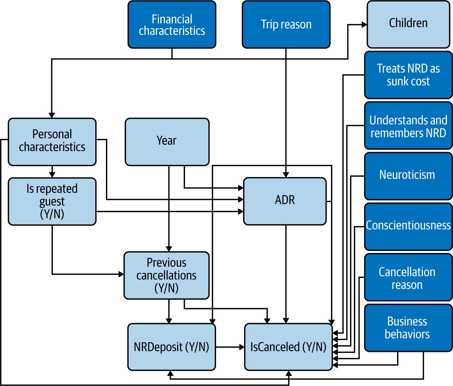
Figure 4-18. Tentatively complete CD with observable and unobservable variables, grouping personal characteristics variables under one heading for readability
From there, we’ll expand our CD iteratively by identifying proxies for unobserved variables and identifying further causes of the current variables.
Identify Proxies for Unobserved Variables
Unobserved variables represent a challenge, because even if they are confirmed through interviews or UX research, they can’t be accounted for directly in the regression analysis.
We can still try to mitigate them somewhat by identifying potential proxies through interviews and research. For example, we may find that conscientiousness is indeed correlated with a lower rate of cancellation, but also with requesting a confirmation email (Figure 4-19).
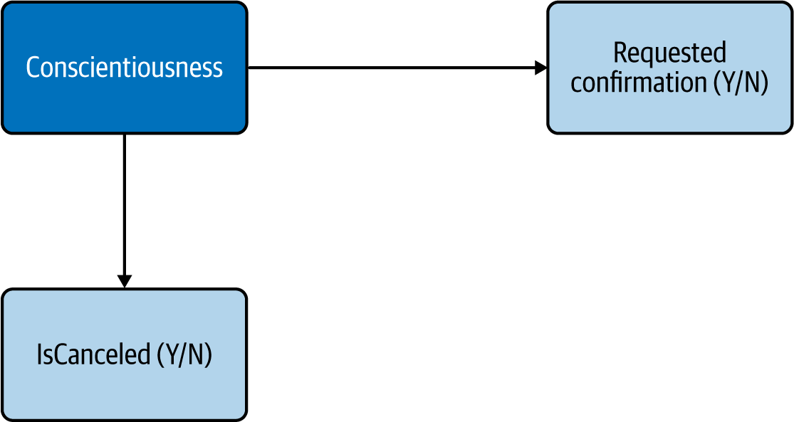
Figure 4-19. Identifying proxies for unobserved variables
Of course, requesting a confirmation email is not caused only by conscientiousness—it may also reflect the seriousness of the intent, lack of ease with digital channels, etc. And conversely, it may reduce the cancellation rate by itself, by providing easily accessible information on the reservation. Regardless, if we find that this behavior is negatively correlated with cancellation rate, we may leverage that insight by, for example, sending an SMS reminder to customers who didn’t choose to receive a confirmation email.
By brainstorming and validating through research potential proxies for unobserved variables, we’re providing meaningful connections between observable variables. Knowing that RequestedConfirmation is connected with IsCanceled through Conscientiousness provides a behavioral rationale for what would otherwise be a raw statistical regularity.
Identify Further Causes
We’ll also expand our CD by identifying causes of the “outer” variables in our CD, i.e., the variables that currently don’t have any parent in our CD. In particular, when we have a variable A that affects our cause of interest (possibly indirectly) but not our effect of interest, and another variable B that conversely affects our effect of interest but not our cause of interest, any joint cause of A and B introduces confounding in our CD, because that joint cause is also a joint cause of our two variables of interest.
In our example, the only observable variable without any parent (observable or not) is Year, and obviously it can’t have one (apart maybe from the laws of physics?), so this step doesn’t apply.
Iterate
As you introduce new variables, you create new opportunities for proxies and further causes. For example, our newly introduced RequestedConfirmation may be affected by Conscientiousness but also by TripReason. This means you should continue to expand your CD until it appears to account for all the relevant variables that you can think of and their interconnections.
There are however significant decreasing returns to this process: as you expand your CD “outward,” the newly added variables will tend to have smaller and smaller correlations with your variables of interest, because of all the noise along the way. This means that accounting for them will deconfound your relationship of interest in smaller and smaller quantities.
Simplify Causal Diagram
The final step once you’ve decided to stop iteratively expanding the CD is to simplify it. Indeed, you now have a diagram that is hopefully accurate and complete for practical purposes, but it might not be structured in the way that would be most helpful to meet the needs of the business. Therefore I would recommend the following simplification steps:
-
Collapse chains when the intermediary variables are not of interest or are unobserved.
-
Expand chains when you need to find observed variables or if you want to track the way another variable relates to the diagram.
-
Slice variables when you think the individual variables would contain interesting information (e.g., the correlation with one of your variables of interest is really driven by only one slice in particular).
-
Combine variables for clarity when reading the diagram or when variation between types does not matter.
-
Break cycles wherever you find them by introducing intermediary steps or identifying the aspect of the relationship that is important.
In our example, we may decide that IsRepeatedGuest, Children, and Year do not add value beyond what is captured through PreviousCancellation and ADR. Indeed, we can dispense with these three variables because they can’t confound our relationship of interest (Figure 4-20).
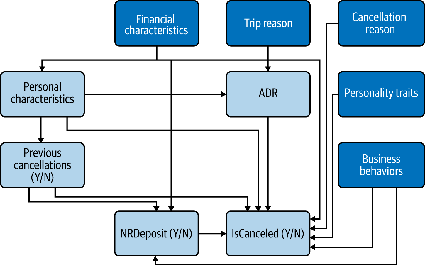
Figure 4-20. Final CD after simplification
You should be left with a clean and (somewhat!) readable diagram, although it might be somewhat larger than those we have seen so far.
If this process seems long and somewhat tedious, that’s because it is. Understanding your business very well is the price to pay to be able to draw causal inferences on customer (or employee) behavior that are at least somewhat valid when you are not able to run experiments.
Fortunately, this process is extremely cumulative and transferable. Once you’ve done it for a certain analysis, your knowledge of the causal relationships that matter for your business can be reused for another analysis. Even if you don’t go very deep the first time you go through this process, you can just focus on one category of confounders and causes; the next time you run this analysis or a similar one, you can pick up where you left and do a deeper dive on another category, maybe interviewing customers about a different aspect of their experience. Similarly, once someone has gone through the process, a new team member or employee can very easily and quickly acquire the corresponding knowledge and pick up where they left off by looking at the resulting CD or even just the list of relevant variables to keep in mind.
Conclusion
To use the cliche phrase, building a CD is an art and a science. I have done my best to provide as clear a recipe as possible to do so:
-
Start with the relationship that you’re trying to measure.
-
Identify candidate variables to include. Namely, use your behavioral science knowledge and business expertise to identify variables that are likely affecting either of your variables of interest.
-
Confirm which observable variables to include based on their correlations in the data.
-
Iteratively expand your CD by adding proxies for unobserved variables where possible and adding further causes of the variables included so far.
-
Finally, simplify your CD by removing irrelevant relationships and variables.
As you do so, always keep in mind your ultimate goal: measuring the causal impact of your cause of interest on your effect of interest. We’ll see in the next chapter how to use a CD to remove confounding in your analysis and obtain an unbiased estimate for that impact. Thus, the best CD is the one that allows you to make the best use of the data you currently have available and that drives fruitful further research.
1 Nuno Antonio, Ana de Almeida, and Luis Nunes, “Hotel booking demand data sets,” Data in Brief, 2019. https://doi.org/10.1016/j.dib.2018.11.126
2 This colorful label was popularized by behavioral scientist Daniel Kahneman.
3 Think about it: how would the rule be implemented otherwise?
Get Behavioral Data Analysis with R and Python now with the O’Reilly learning platform.
O’Reilly members experience books, live events, courses curated by job role, and more from O’Reilly and nearly 200 top publishers.

