Data Science on the Google Cloud Platform

Chapter 4. Streaming Data: Publication and Ingest

In Chapter 3, we developed a dashboard to explain a contingency table–based model of suggesting whether to cancel a meeting. However, the dashboard that we built lacked immediacy because it was not tied to users’ context. Because users need to be able to view a dashboard and see the information that is relevant to them at that point, we need to build a real-time dashboard with location cues.

How would we add context to our dashboard? We’d have to show maps of delays in real time. To do that, we’ll need locations of the airports, and we’ll need real-time data. Airport locations can be obtained from the US Bureau of Transportation Statistics (BTS; the same US government agency from which we obtained our historical flight data). Real-time flight data, however, is a commercial product. If we were to build a business out of predicting flight arrivals, we’d purchase that data feed. For the purposes of this book, however, let’s just simulate it.

Simulating the creation of a real-time feed from historical data has the advantage of allowing us to see both sides of a streaming pipeline (production as well as consumption). In the following section, we look at how we could stream the ingest of data into the database if we were to receive it in real time.

Designing the Event Feed

To create a real-time stream of flight information, we begin by using historical data that is appropriately transformed from what we downloaded from the BTS. What kinds of transformations are needed?

The historical data has this structure:

FL_DATE,UNIQUE_CARRIER,AIRLINE_ID,CARRIER,FL_NUM,ORIGIN_AIRPORT_ID,
ORIGIN_AIRPORT_SEQ_ID,ORIGIN_CITY_MARKET_ID,ORIGIN,DEST_AIRPORT_ID,
DEST_AIRPORT_SEQ_ID,DEST_CITY_MARKET_ID,DEST,CRS_DEP_TIME,DEP_TIME,
DEP_DELAY,TAXI_OUT,WHEELS_OFF,WHEELS_ON,TAXI_IN,CRS_ARR_TIME,
ARR_TIME,ARR_DELAY,CANCELLED,CANCELLATION_CODE,DIVERTED,DISTANCE

An example row of the historical data in the comma-separated value (CSV) file looks like this:

2015-01-01,AA,19805,AA,1,12478,1247802,31703,JFK,12892,1289203,32575,LAX,0900,
0855,-5.00,17.00,0912,1230,7.00,1230,1237,7.00,0.00,,0.00,2475.00

To simulate real-time behavior, we need to key off the timestamps in the historical data. The departure time is present in the BTS flights dataset in the form of two columns: FL_DATE and DEP_TIME (bolded in the example). The FL_DATE is of the form 2015-07-03 for July 3, 2015, and DEP_DATE is of the form 1406 for 2:06 PM local time. This is unfortunate. I’m not worried about the separation of date and time into two columns—we can remedy that. What’s unfortunate is that there is no time zone offset associated with the departure time. Thus, in this dataset, a departure time of 1406 in different rows can be different times depending on the time zone of the origin airport.

The time zone offsets (there are two, one for the origin airport and another for the destination) are not present in the data. Because the offset depends on the airport location, we need to find a dataset that contains the timezone offset of each airport and then mash this data with that dataset.¹ To simplify downstream analysis, we will then put all the times in the data in a common time zone—Coordinated Universal Time (UTC) is the traditional choice of common time zone for datasets. We cannot however, get rid of the local time—we will need the local time in order to carry out analysis, such as the typical delay associated with morning flights versus evening flights. So, although we will convert the local times to UTC, we will also store the time zone offset (e.g., –3,600 minutes) to retrieve the local time if necessary.

Therefore, we are going to carry out two transformations to the original dataset. First, we will convert all the time fields in the raw dataset to UTC. Secondly, in addition to the fields present in the raw data, we will add three fields to the dataset for the origin airport and the same three fields for the destination airport: the latitude, longitude, and time zone offset. These fields will be named:

DEP_AIRPORT_LAT, DEP_AIRPORT_LON, DEP_AIRPORT_TZOFFSET

ARR_AIRPORT_LAT, ARR_AIRPORT_LON, ARR_AIRPORT_TZOFFSET

The third transformation that we will need to carry out is that for every row in the historical dataset, we will need to publish multiple events. This is because it would be too late if we wait until the aircraft has arrived to send out a single event containing all the row data. If we do this at the time the aircraft departs, our models will be violating causality constraints. Instead, we will need to send out events corresponding to each state the flight is in. Let’s choose to send out five events for each flight: when the flight is first scheduled, when the flight departs the gate, when the flight lifts off, when the flight lands, and when the flight arrives. These five events cannot have all the same data associated with them because the knowability of the columns changes during the flight. For example, when sending out an event at the departure time, we will not know the arrival time. For simplicity, we can notify the same structure, but we will need to ensure that unknowable data is marked by a null and not with the actual data value.

Table 4-1 lists when those events can be sent out and the fields that will be included in each event.

Table 4-1. Fields that will be included in each of the five events that will be published

Event	Sent at (UTC)	Fields included in event message
Scheduled	CRS_DEP_TIME minus 7 days	FL_DATE,UNIQUE_CARRIER,AIRLINE_ID,CARRIER,FL_NUM,ORIGIN_AIRPORT_ID, ORIGIN_AIRPORT_SEQ_ID,ORIGIN_CITY_MARKET_ID,ORIGIN,DEST_AIRPORT_ID, DEST_AIRPORT_SEQ_ID,DEST_CITY_MARKET_ID,DEST,CRS_DEP_TIME, [nulls],CRS_ARR_TIME,[nulls],DISTANCE,[nulls]
Departed	DEP_TIME	All fields available in scheduled message, plus: DEP_TIME,DEP_DELAY CANCELLED,CANCELLATION_CODE DEP_AIRPORT_LAT,DEP_AIRPORT_LON,DEP_AIRPORT_TZOFFSET
Wheelsoff	WHEELS_OFF	All fields available in departed message, plus: TAXI_OUT,WHEELS_OFF
Wheelson	WHEELS_ON	All fields available in wheelsoff message, plus: WHEELS_ON DIVERTED ARR_AIRPORT_LAT,ARR_AIRPORT_LON,ARR_AIRPORT_TZOFFSET
Arrived	ARR_TIME	All fields available in wheelson message, plus: ARR_TIME,ARR_DELAY

We will carry out the transformations needed and then store the transformed data in a database so that it is ready for the event simulation code to use. Figure 4-1 shows the steps we are about to carry out in our Extract-Transform-Load (ETL) pipeline.

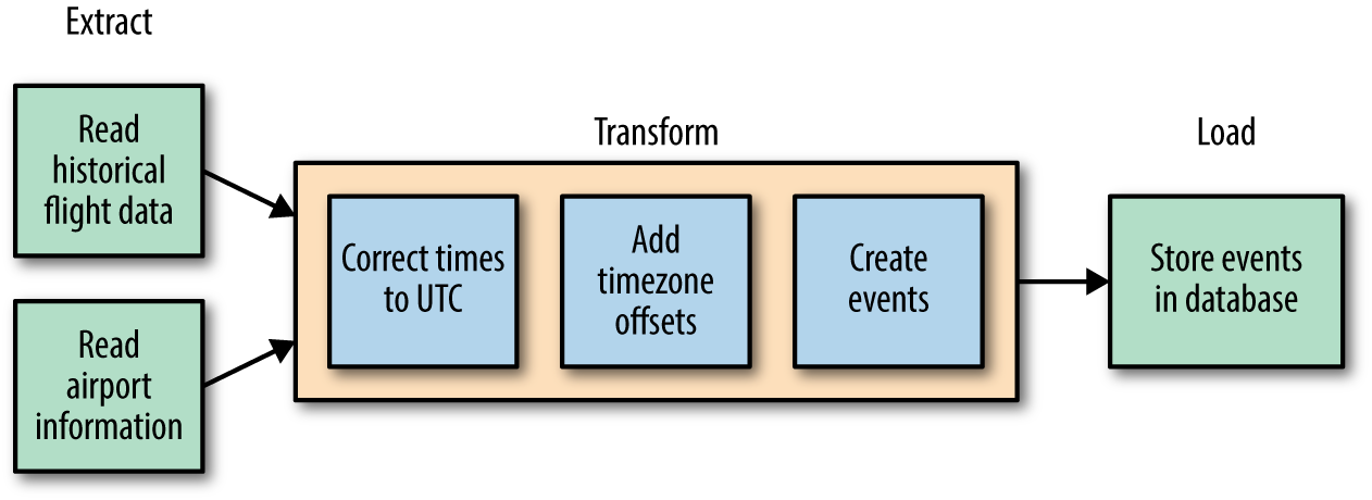
Figure 4-1. Steps in our ETL pipeline

Time Correction

Correcting times reported in local time to UTC is not a simple endeavor. There are several steps:

1. Local time depends on, well, the location. The flight data that we have records only the name of the airport (ALB for Albany). We, therefore, need to obtain the latitude and longitude given an airport code. The BTS has a dataset that contains this information, which we can use to do the lookup.

2. Given a latitude/longitude pair, we need to look up the time zone from a map of global time zones. For example, given the latitude and longitude of the airport in Albany, we would need to get back America/New_York. There are several web services that do this, but the Python package timezonefinder is a more efficient option because it works completely offline. The drawback is that this package does not handle oceanic areas and some historical time zone changes,² but that’s a trade-off that we can make for now.

3. The time zone offset at a location changes during the year due to daylight savings corrections. In New York, for example, it is six hours in summer and five hours in winter. Given the time zone (America/New_York), therefore, we also need the local departure date and time (say Jan 13, 2015 2:08 PM) in order to find the corresponding time zone offset. The Python package pytz provides this capability by using the underlying operating system.

The problem of ambiguous times still remains—every instant between 01:00 and 02:00 local time occurs twice on the day that the clock switches from daylight savings time (summer time) to standard time (winter time). So, if our dataset has a flight arriving at 01:30, we need to make a choice of what time that represents. In a real-world situation, you would look at the typical duration of the flight and choose the one that is more likely. For the purposes of this book, I’ll always assume the winter time (i.e., is_dst is False) on the dubious grounds that it is the standard time zone for that location.

The complexity of these steps should, I hope, convince you to follow best practices when storing time. Always try to store two things in your data: (1) the timestamp in UTC so that you can merge data from across the world if necessary and (2) the currently active time zone offset so that you can carry out analysis that requires the local time.³

Apache Beam/Cloud Dataflow

The canonical way to build data pipelines on Google Cloud Platform is to use Cloud Dataflow. Cloud Dataflow is an externalization of technologies called Flume and Millwheel that have been in widespread use at Google for several years. It employs a programming model that handles both batch and streaming data in a uniform manner, thus providing the ability to use the same code base both for batch and continuous stream processing. The code itself is written in Apache Beam, either in Java or Python,⁴ and is portable in the sense that it can be executed on multiple execution environments including Apache Flink⁵ and Apache Spark. On Google Cloud Platform, Cloud Dataflow provides a fully managed (serverless) service that is capable of executing Beam pipelines. Resources are allocated on-demand and they autoscale so as to achieve both minimal latency and high resource utilization.

Beam programming involves building a pipeline (a series of data transformations) that is submitted to a runner. The runner will build a graph and then stream data through it. Each input dataset comes from a source and each output dataset is sent to a sink. Figure 4-2 illustrates the Beam pipeline that we are about to build.

Compare the steps in Figure 4-2 with the block diagram of the ETL pipeline at the beginning of this section in Figure 4-1. Let’s build the data pipeline piece by piece.

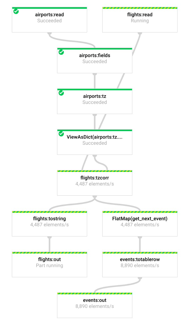
Figure 4-2. The Dataflow pipeline that we are about to build

Parsing Airports Data

You can download information about the location of airports from the BTS website. I selected all of the fields, downloaded it to my local hard drive, extracted the CSV file, and compressed it with gzip. The gzipped airports file is available in the GitHub repository for this book.

The Read transform in the Beam pipeline that follows reads in the airports file line by line.⁶

   with beam.Pipeline('DirectRunner') as pipeline:
      airports = (pipeline
         | beam.io.ReadFromText('airports.csv.gz')
         | beam.Map(lambda line: next(csv.reader([line])))
         | beam.Map(lambda fields: (fields[0], (fields[21], fields[26])))
      )

For example, suppose that one of the input lines read out of the text file source is the following:

1000401,10004,"04A","Lik Mining Camp","Lik, AK",101,1,"United
States","US","Alaska","AK","02",3000401,30004,"Lik,
AK",101,1,68,"N",5,0,68.08333333,163,"W",10,0,-163.16666667,"",2007-07-01,,0,1,

The first Map takes this line and passes it to a CSV reader that parses it (taking into account fields like "Lik, AK" that have commas in them) and pulls out the fields as a list of strings. These fields are then passed to the next transform. The second Map takes the fields as input and outputs a tuple of the form (the extracted fields are shown in bold in the previous example):

(1000401, (68.08333333,-163.16666667))

The first number is the unique airport code (we use this, rather than the airport’s three-letter code, because airport locations can change over time) and the next two numbers are the latitude/longitude pair for the airport’s location. The variable airports, which is the result of these three transformations, is not a simple in-memory list of these tuples. Instead, it is an immutable collection, termed a PCollection, that you can take out-of-memory and distribute.

We can write the contents of the PCollection to a text file to verify that the pipeline is behaving correctly:

(airports
   | beam.Map(lambda airport_data: '{},{}'.format(airport_data[0], ',' \
       .join(airport_data[1])) )
   | beam.io.WriteToText('extracted_airports')
)

Try this out: the code, in 04_streaming/simulate/df01.py, is just a Python program that you can run from the command line. First, install the Apache Beam package (Cloud Dataflow is an execution environment for Apache Beam) and then run the program df01.py while you are in the directory containing the GitHub repository of this book:

cd 04_streaming/simulate
./install_packages.sh
python3 ./df01.py

This runs the code in df01.py locally. Later, we will change the pipeline line to:

   with beam.Pipeline('DataflowRunner') as pipeline:

and get to run the pipeline on the Google Cloud Platform using the Cloud Dataflow service. With that change, simply running the Python program launches the data pipeline on multiple workers in the cloud. As with many distributed systems, the output of Cloud Dataflow is potentially sharded to one or more files. You will get a file whose name begins with “extracted_airports” (mine was extracted_airports-00000-of-00001), a few of whose lines might look something like this:

1000101,58.10944444,-152.90666667
1000301,65.54805556,-161.07166667

The columns are AIRPORT_SEQ_ID,LATITUDE,LONGITUDE—the order of the rows you get depends on which of the parallel workers finished first, and so could be different.

Adding Time Zone Information

Let’s now change the code to determine the time zone corresponding to a latitude/longitude pair. In our pipeline, rather than simply emitting the latitude/longitude pair, we emit a list of three items: latitude, longitude, and time zone:

airports = (pipeline
      | beam.Read(beam.io.ReadFromText('airports.csv.gz'))
      | beam.Map(lambda line: next(csv.reader([line])))
      | beam.Map(lambda fields: (fields[0], addtimezone(fields[21], fields[26])))
   )

The lambda keyword in Python sets up an anonymous function. In the case of the first use of lambda in the above snippet, that method takes one parameter (line) and returns the stuff following the colon. We can determine the time zone by using the timezonefinder package:⁷

def addtimezone(lat, lon):
   try:
      import timezonefinder
      tf = timezonefinder.TimezoneFinder()
      tz = tf.timezone_at(lng=float(lon), lat=float(lat)) # throws ValueError
      if tz is None:
         tz = 'UTC'
      return (lat, lon, tz)
   except ValueError:
      return (lat, lon, 'TIMEZONE') # header

The location of the import statement in the preceding example might look strange (most Python imports tend to be at the top of the file), but is recommended by Cloud Dataflow⁸ so that pickling of the main session when we finally do submit it to the cloud doesn’t end up pickling imported packages, also.

For now, though, we are going to run this (df02.py) locally. This will take a while⁹ because the time zone computation involves a large number of polygon intersection checks and because we are running locally, not (yet!) distributed in the cloud. The extracted information now looks like this:

1000101,58.10944444,-152.90666667,America/Anchorage
1000301,65.54805556,-161.07166667,America/Anchorage
1000401,68.08333333,-163.16666667,America/Nome

The last column now has the time zone, which was determined from the latitude and longitude of each airport.

Converting Times to UTC

Now that we have the time zone for each airport, we are ready to tackle converting the times in the flights data to UTC. While we are developing the program, we’d prefer not to process all the months we have in Cloud Storage. Instead, we will create a small sample of the flights data against which to try our code:

gsutil cat gs://cloud-training-demos-ml/flights/raw/201501.csv \
                           | head -1000 > 201501_part.csv

The 201501_part.csv file contains 1,000 lines, which is enough to test the pipeline against locally.

Reading the flights data starts out similar to reading the airports data:¹⁰

flights = (pipeline
  | 'flights:read' >> beam.io.ReadFromText('201501_part.csv')

This is the same code as when we read the airports.csv.gz file, except that I am also giving a name (flights:read) to this transform step.

The next step, though, is different because it involves two PCollections. We need to join the flights data with the airports data to find the time zone corresponding to each flight. To do that, we make the airports PCollection a “side input.” Side inputs in Beam are like views into the original PCollection, and are either lists or dicts. In this case, we will create a dict that maps airport ID to information about the airports:

flights = (pipeline
 |'flights:read' >> beam.io.ReadFromText('201501_part.csv')
 |'flights:tzcorr' >> beam.FlatMap(tz_correct, beam.pvalue.AsDict(airports))
)

The FlatMap() method calls out to a method tz_correct(), which takes a line from 201501_part.csv (containing a single flight’s information) and a Python dictionary (containing all the airports’ time zone information):

def tz_correct(line, airport_timezones):
   fields = line.split(',')
   if fields[0] != 'FL_DATE' and len(fields) == 27:
      # convert all times to UTC
      dep_airport_id = fields[6]
      arr_airport_id = fields[10]
      dep_timezone = airport_timezones[dep_airport_id][2]
      arr_timezone = airport_timezones[arr_airport_id][2]
     
      for f in [13, 14, 17]: #crsdeptime, deptime, wheelsoff
         fields[f] = as_utc(fields[0], fields[f], dep_timezone)
      for f in [18, 20, 21]: #wheelson, crsarrtime, arrtime
         fields[f] = as_utc(fields[0], fields[f], arr_timezone)
    
      yield ','.join(fields)

Why FlatMap() instead of Map to call tz_correct()? A Map is a 1-to-1 relation between input and output, whereas a FlatMap() can return 0–N outputs per input. The way it does this is with a Python generator function (i.e., the yield keyword—think of the yield as a return that returns one item at a time until there is no more data to return).

The tz_correct() code gets the departure airport ID from the flight’s data and then looks up the time zone for that airport ID from the airport’s data. After it has the time zone, it calls out to the method as_utc() to convert each of the date–times reported in that airport’s time zone to UTC:

def as_utc(date, hhmm, tzone):
   try:
      if len(hhmm) > 0 and tzone is not None:
         import datetime, pytz
         loc_tz = pytz.timezone(tzone)
         loc_dt = loc_tz.localize(datetime.datetime.strptime(date,'%Y-%m-%d'),
                                  is_dst=False)
         loc_dt += datetime.timedelta(hours=int(hhmm[:2]),
                                      minutes=int(hhmm[2:]))
         utc_dt = loc_dt.astimezone(pytz.utc)
         return utc_dt.strftime('%Y-%m-%d %H:%M:%S')
      else:
         return '' # empty string corresponds to canceled flights
   except ValueError as e:
      print('{} {} {}'.format(date, hhmm, tzone))
      raise e

As before, you can run this locally. To do that, run df03.py. A line that originally (in the raw data) looked like

2015-01-01,AA,19805,AA,8,12173,1217302,32134,HNL,11298,1129803,30194,DFW,1745,
1933,108.00,15.00,1948,0648,11.00,0510,0659,109.00,0.00,,0.00,3784.00

now becomes:

2015-01-01,AA,19805,AA,8,12173,1217302,32134,HNL,11298,1129803,30194,DFW,2015-01-
02 03:45:00,2015-01-02 05:33:00,108.00,15.00,2015-01-02 05:48:00,
2015-01-01 12:48:00,11.00,2015-01-01 11:10:00,2015-01-01 
12:59:00,109.00,0.00,,0.00,3784.00

All the times have been converted to UTC. For example, the 0648 time of arrival in Dallas has been converted to UTC to become 12:48:00.

Correcting Dates

Look carefully at the previous line involving a flight from Honolulu (HNL) to Dallas–Fort Worth (DFW). Do you notice anything odd?

Carefully take a look at the departure time in Honolulu and the arrival time in Dallas:

2015-01-01,AA,19805,AA,8,12173,1217302,32134,HNL,11298,1129803,30194,DFW,
2015-01-02 03:45:00,2015-01-02 05:33:00,108.00,15.00,
2015-01-02 05:48:00,2015-01-01 12:48:00,11.00,2015-01-01 11:10:00,
2015-01-01 12:59:00,109.00,0.00,,0.00,3784.00

The flight is arriving the day before it departed! That’s because the flight date (2015-01-01) is the date of departure in local time. Add in a time difference between airports, and it is quite possible that it is not the date of arrival. We’ll look for these situations and add 24 hours if necessary. This is, of course, quite a hack (have I already mentioned that times ought to be stored in UTC?!):

def add_24h_if_before(arrtime, deptime):
   import datetime
   if len(arrtime) > 0 and len(deptime) > 0 and arrtime < deptime:
      adt = datetime.datetime.strptime(arrtime, '%Y-%m-%d %H:%M:%S')
      adt += datetime.timedelta(hours=24)
      return adt.strftime('%Y-%m-%d %H:%M:%S')
   else:
      return arrtime

The 24-hour hack is called just before the yield in tz_correct.¹¹ Now that we have new data about the airports, it is probably wise to add it to our dataset. Also, as remarked earlier, we want to keep track of the time zone offset from UTC because some types of analysis might require knowledge of the local time. Thus, the new tz_correct code becomes the following:

def tz_correct(line, airport_timezones):
   fields = line.split(',')
   if fields[0] != 'FL_DATE' and len(fields) == 27:
      # convert all times to UTC
      dep_airport_id = fields[6]
      arr_airport_id = fields[10]
      dep_timezone = airport_timezones[dep_airport_id][2]
      arr_timezone = airport_timezones[arr_airport_id][2]
     
      for f in [13, 14, 17]: #crsdeptime, deptime, wheelsoff
         fields[f], deptz = as_utc(fields[0], fields[f], dep_timezone)
      for f in [18, 20, 21]: #wheelson, crsarrtime, arrtime
         fields[f], arrtz = as_utc(fields[0], fields[f], arr_timezone)
     
      for f in [17, 18, 20, 21]:
         fields[f] = add_24h_if_before(fields[f], fields[14])

      fields.extend(airport_timezones[dep_airport_id])
      fields[-1] = str(deptz)
      fields.extend(airport_timezones[arr_airport_id])
      fields[-1] = str(arrtz)

      yield ','.join(fields)

Creating Events

After we have our time-corrected data, we can move on to creating events. We’ll limit ourselves for now to just the departed and arrived messages—we can rerun the pipeline to create the additional events if and when our modeling efforts begin to use other events:

def get_next_event(fields):
    if len(fields[14]) > 0:
       event = list(fields) # copy
       event.extend(['departed', fields[14]])
       for f in [16,17,18,19,21,22,25]:
          event[f] = ''  # not knowable at departure time
       yield event
    if len(fields[21]) > 0:
       event = list(fields)
       event.extend(['arrived', fields[21]])
       yield event

Essentially, we pick up the departure time and create a departed event at that time after making sure to null out the fields we cannot know at the departure time. Similarly, we use the arrival time to create an arrived event. In the pipeline, this is called on the flights PCollection after the conversion to UTC has happened:

flights = (pipeline
  |'flights:read' >> beam.io.ReadFromText('201501_part.csv')
  |'flights:tzcorr' >> beam.FlatMap(tz_correct, beam.pvalue.AsDict(airports))
)
events = flights | beam.FlatMap(get_next_event)

If we now run the pipeline,¹² we will see two events for each flight:

2015-01-01,AA,19805,AA,1,12478,1247802,31703,JFK,12892,1289203,32575,LAX,2015-01-
01T14:00:00,2015-01-01T13:55:00,-5.00,,,,,2015-01-01T20:30:00,,,0.00,,,
2475.00,40.63972222,-73.77888889,-18000.0,33.94250000,-118.40805556,
-28800.0,departed,2015-01-01T13:55:00
2015-01-01,AA,19805,AA,1,12478,1247802,31703,JFK,12892,1289203,32575,LAX,2015-01-
01T14:00:00,2015-01-01T13:55:00,-5.00,17.00,2015-01-01T14:12:00,2015-01-01
T20:30:00,7.00,2015-01-01T20:30:00,2015-01-01T20:37:00,7.00,0.00,,0.00,
2475.00,40.63972222,-73.77888889,-18000.0,33.94250000,-118.40805556,
-28800.0,arrived,2015-01-01T20:37:00

The first event is a departed event and is to be published at the departure time, while the second is an arrived event and is to be published at the arrival time. The departed event has a number of empty fields corresponding to data that is not known at that time.

Running the Pipeline in the Cloud

That last run took a few minutes on the local virtual machine (VM), and we were processing only a thousand lines! We need to distribute the work, and to do that, we will change the runner from DirectRunner (which runs locally) to DataflowRunner (which lobs the job off to the cloud and scales it out).¹³ We’ll change the input data to be in Cloud Storage (as discussed in Chapter 2, the data is in situ; i.e., we don’t need to preshard the data):

argv = [
      '--project={0}'.format(project),
      '--job_name=ch03timecorr',
      '--save_main_session',
      '--staging_location=gs://{0}/flights/staging/'.format(bucket),
      '--temp_location=gs://{0}/flights/temp/'.format(bucket),
      '--setup_file=./setup.py',
      '--max_num_workers=10',
      '--autoscaling_algorithm=THROUGHPUT_BASED',
      '--runner=DataflowRunner'
   ]
   airports_filename =
        'gs://{}/flights/airports/airports.csv.gz'.format(bucket)
   flights_raw_files = 'gs://{}/flights/raw/*.csv'.format(bucket)
   flights_output = 'gs://{}/flights/tzcorr/all_flights'.format(bucket)
   events_output = '{}:flights.simevents'.format(project)

   pipeline = beam.Pipeline(argv=argv)

The file setup.py should list the Python packages that we needed to install (timezonefinder and pytz) as we went along—Cloud Dataflow will need to install these packages on the Compute Engine instances that it launches behind the scenes:

REQUIRED_PACKAGES = [
    'timezonefinder',
    'pytz'
]

As a final touch, we store the time-corrected flight data as CSV files in Cloud Storage but store the events in BigQuery. BigQuery is Google Cloud Platform’s data warehouse that supports SQL queries and makes it easier if you want to pull out a subset of events to simulate.

Note

We look at BigQuery in more detail in Chapter 5.

To do that, the writing code becomes the following:

schema = 'FL_DATE:date,UNIQUE_CARRIER:string,...'
(events
 | 'events:totablerow' >> beam.Map(lambda fields: create_row(fields))
 | 'events:out' >> beam.io.WriteToBigQuery(
                              events_output, schema=schema,
write_disposition=beam.io.BigQueryDisposition.WRITE_TRUNCATE,
create_disposition=beam.io.BigQueryDisposition.CREATE_IF_NEEDED)
   )

The create_row() method simply creates a dictionary of the fields to be written:

def create_row(fields):
    header = 'FL_DATE,UNIQUE_CARRIER,...'.split(',')
    featdict = {}
    for name, value in zip(header, fields):
        featdict[name] = value
    return featdict

Before you run this program, you need to create a dataset in BigQuery called flights because the simevents table will be created by the pipeline if necessary,¹⁴ but not the dataset. To do that, type the following:

bq mk flights

You also need to upload the airports.csv.gz file from the course repository to your Cloud Storage bucket:

gsutil cp airports.csv.gz \
     gs://<BUCKET-NAME>/flights/airports/airports.csv.gz

Running the Python program with the preceding code¹⁵ submits the job to the cloud. Cloud Dataflow autoscales each step of the pipeline based on throughput, and streams the events data into BigQuery. You can monitor the running job on the Cloud Platform Console in the Cloud Dataflow section.

Even as the events data is being written out, we can query it by browsing to the BigQuery console and typing the following:

SELECT
  ORIGIN,
  DEP_TIME,
  DEP_DELAY,
  DEST,
  ARR_TIME,
  ARR_DELAY,
  NOTIFY_TIME
FROM
  flights.simevents
WHERE
  (DEP_DELAY > 15 and ORIGIN = 'SEA') or
  (ARR_DELAY > 15 and DEST = 'SEA')
ORDER BY NOTIFY_TIME ASC
LIMIT
  10

Figure 4-3 shows what I got when I ran this query.

Figure 4-3. Result of query as events data were being written out

As expected, we see two events for the SEA-IAD flight, one at departure and the other at arrival.

BigQuery is a columnar database, so a query that selects all fields

SELECT
  *
FROM
  flights.simevents
ORDER BY NOTIFY_TIME ASC

will be very inefficient. However, we do need all of the event data in order to send out event notifications. Therefore, we trade off storage for speed by adding an extra column called EVENT_DATA to our BigQuery table and then populate it in our pipeline as follows (we also have to modify the BigQuery schema appropriately):

def create_row(fields):
    header = 'FL_DATE,UNIQUE_CARRIER,...,NOTIFY_TIME'.split(',')

    featdict = {}
    for name, value in zip(header, fields):
        featdict[name] = value
    featdict['EVENT_DATA'] = ','.join(fields)
    return featdict

Then, our query to pull the events could simply be as follows:

SELECT
  EVENT,
  NOTIFY_TIME,
  EVENT_DATA
FROM
  flights.simevents
WHERE
  NOTIFY_TIME >= TIMESTAMP('2015-05-01 00:00:00 UTC')
  AND NOTIFY_TIME < TIMESTAMP('2015-05-03 00:00:00 UTC')
ORDER BY
  NOTIFY_TIME ASC
LIMIT
  10

Figure 4-4 depicts the query results.

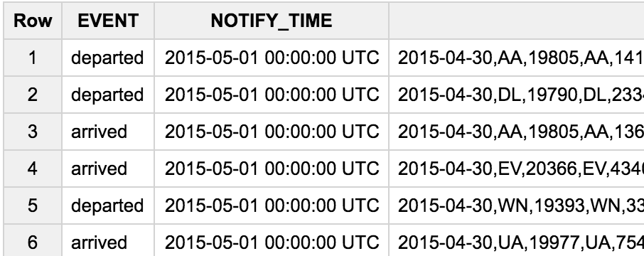
Figure 4-4. Query result with the additional EVENT_DATA field

This table will serve as the source of our events; it is from such a query that we will simulate streaming flight data.

Publishing an Event Stream to Cloud Pub/Sub

Now that we have the source events from the raw flight data, we are ready to simulate the stream. Streaming data in Google Cloud Platform is typically published to Cloud Pub/Sub, a serverless real-time messaging service. Cloud Pub/Sub provides reliable delivery and can scale to more than a million messages per second. It stores copies of messages in multiple zones to provide “at least once” guaranteed delivery to subscribers, and there can be many simultaneous subscribers.

Our simulator will read from the events table in BigQuery (populated in the previous section) and publish messages to Cloud Pub/Sub based on a mapping between the event notification time (arrival or departure time based on event) and the current system time, as illustrated in Figure 4-5.

Essentially, we will walk through the flight event records, getting the notification time from each.

It is inefficient to always simulate the flights events at real-time speeds. Instead, we might want to run through a day of flight data in an hour (as long as the code that processes these events can handle the increased data rate). At other times, we may be running our event-processing code in a debugging environment that is slower and so we might want to slow down the simulation. I will refer to this ratio between the actual time and simulation time as the speed-up factor—the speed-up factor will be greater than 1 if we want the simulation to be faster than real time, and less than 1 if we want it to be slower than real time.

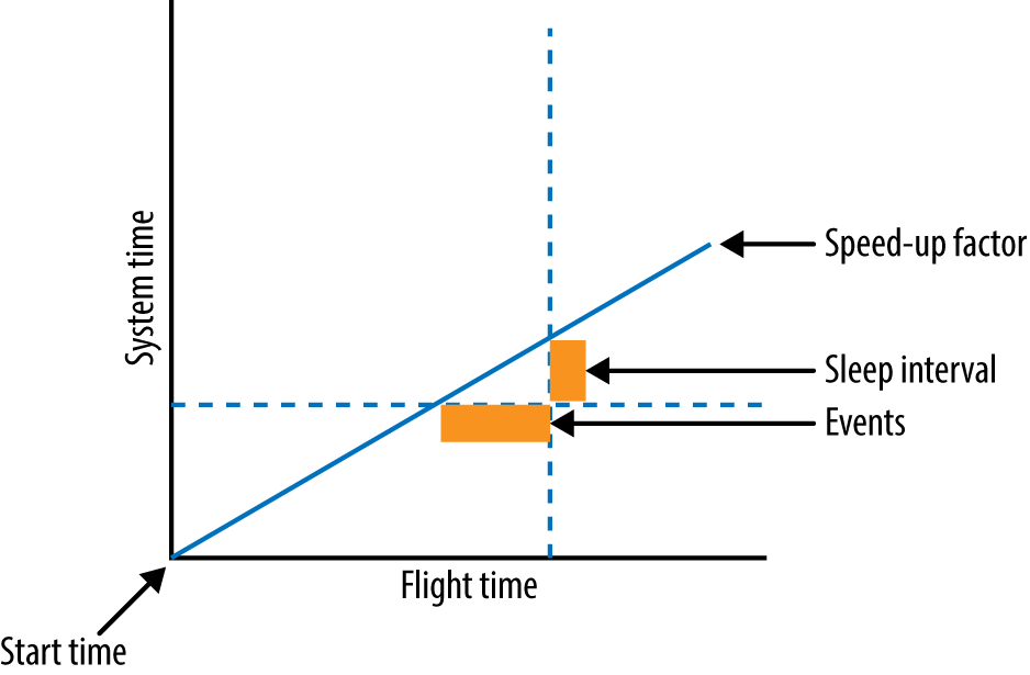
Figure 4-5. The simulator publishes messages based on a mapping between event time and system time

Based on the speed-up factor, we’ll have to do a linear transformation of the event time to system time. If the speed-up factor is 1, a 60-minute difference between the start of the simulation in event time and the current record’s timestamp should be encountered 60 minutes after the start of the simulation. If the speed-up factor is 60, a 60-minute difference in event time translates to a 1-minute difference in system time, and so the record should be published a minute later. If the event time clock is ahead of the system clock, we sleep for the necessary amount of time so as to allow the simulation to catch up.

The simulation consists of four steps (see also Figure 4-6).¹⁶

1. Run the query to get the set of flight event records to publish.

2. Page through the query.

3. Accumulate events to publish as a batch.

4. Publish accumulated events and sleep as necessary.

Even though this is an ETL pipeline, the need to process records in strict sequential order and sleep in between makes this ETL pipeline a poor fit for Cloud Dataflow. Instead, we’ll implement this as a pure Python program. The problem with this choice is that the simulation code is not fault tolerant—if the simulation fails, it will not automatically restart and definitely will not start from the last successfully notified event.

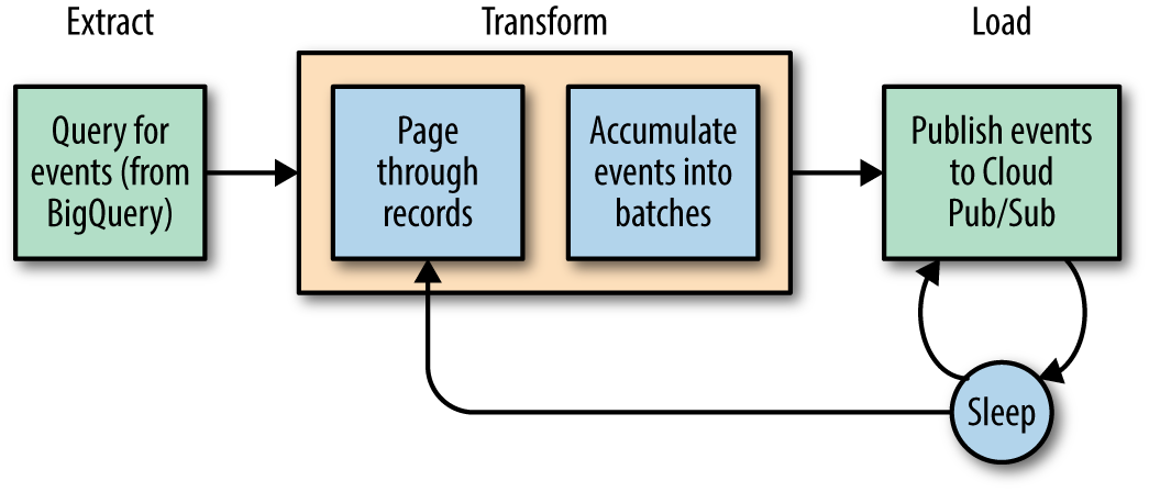
Figure 4-6. The four steps of simulation

The simulation code that we are writing is only for quick experimentation with streaming data. Hence, I will not take the extra effort needed to make it fault-tolerant. If we had to do so, we could make the simulation fault-tolerant by starting from a BigQuery query that is bounded in terms of a time range with the start of that time range automatically inferred from the last-notified record in Cloud Pub/Sub. Then, we could launch the simulation script from a Docker container and use Cloud Run or Google Container Engine (which runs Kubernetes) to automatically restart the simulation if the simulation code fails. All this, though, strikes me as gilding the lily—for quick experimentation, it is unclear whether the code needs to be fault-tolerant. For now, therefore, let’s note that the simulation code as written will not automatically restart, and even if manually restarted, it will not resume where it last left off.¹⁷ If we need to make the simulator enterprise-grade, we can revisit this.

Get Records to Publish

The BigQuery query is parameterized by the start and end time of the simulation and can be invoked through the Google Cloud API for Python:

   bqclient = bq.Client() 
   # run the query to pull simulated events
   querystr = """
SELECT
  EVENT,
  NOTIFY_TIME,
  EVENT_DATA
FROM
  flights.simevents
WHERE
  NOTIFY_TIME >= TIMESTAMP('{}')
  AND NOTIFY_TIME < TIMESTAMP('{}')
ORDER BY
  NOTIFY_TIME ASC
   """
   rows = bqclient.query(querystr.format(args.startTime,
                                         args.endTime))
   for row in rows:
     # do something

We get back an object (called rows in the above snippet) that we can iterate through.

Paging Through Records

As we walk through the query results, we need to publish to Cloud Pub/Sub. There is a separate topic per event type (i.e., an arrived topic and a departed topic), so we create two topics:

publisher = pubsub.PublisherClient()
topics = {}
for event_type in ['departed', 'arrived']:
    topics[event_type] = publisher.topic_path(args.project, event_type)
    publisher.create_topic(topics[event_type])

After creating the topics, we call the notify() method passing along the rows read from BigQuery:

# notify about each row in the dataset
programStartTime = datetime.datetime.utcnow()
simStartTime = datetime.datetime.strptime(args.startTime, 
                    TIME_FORMAT).replace(tzinfo=pytz.UTC)
notify(publisher, topics, rows, simStartTime, programStartTime, args.speedFactor)

Building a Batch of Events

The notify() method consists of accumulating the rows into batches and publishing them when it is time to sleep:

def notify(publisher, topics, rows, simStartTime, programStart, speedFactor):
   # sleep computation
   def compute_sleep_secs(notify_time):
        time_elapsed = (datetime.datetime.utcnow() - programStart).seconds
        sim_time_elapsed = (notify_time - simStartTime).seconds / speedFactor
        to_sleep_secs = sim_time_elapsed - time_elapsed
        return to_sleep_secs

   tonotify = {}
   for key in topics:
     tonotify[key] = list()

   for row in rows:
       event, notify_time, event_data = row

       # how much time should we sleep?
       if compute_sleep_secs(notify_time) > 1:
          # notify the accumulated tonotify
          publish(publisher, topics, tonotify)
          for key in topics:
             tonotify[key] = list()

          # recompute sleep, since notification takes a while
          to_sleep_secs = compute_sleep_secs(notify_time)
          if to_sleep_secs > 0:
             logging.info('Sleeping {} seconds'.format(to_sleep_secs))
             time.sleep(to_sleep_secs)
 
       tonotify[event].append(event_data)
   # left-over records; notify again
   publish(publisher, topics, tonotify)

There are a few points to be made here. First is that we work completely in UTC so that the time difference computations make sense. We also notify to Cloud Pub/Sub in batches. This is important because notifying to Cloud Pub/Sub involves a network call and is subject to latency—we should minimize that if we can. Otherwise, we’ll be limited in what speed-up factors we can support. Thirdly, we always compute whether to sleep by looking at the time difference since the start of the simulation. If we simply keep moving a pointer forward, errors in time will accumulate. Finally, note that we check whether the sleep time is more than a second the first time, so as to give records time to accumulate. If, when you run the program, you do not see any sleep, your speed-up factor is too high for the capability of the machine running the simulation code and the network between that machine and Google Cloud Platform. Slow down the simulation, get a larger machine, or run it behind the Google firewall (such as on a Compute Engine instance).

Publishing a Batch of Events

The notify() method that we saw in the previous code example has accumulated the events in between sleep calls. Even though it appears that we are publishing one event at a time, the publisher actually maintains a separate batch for each topic:

def publish(publisher, topics, allevents):
   for key in topics:  # 'departed', 'arrived', etc.
      topic = topics[key]
      events = allevents[key]
      logging.info('Publishing {} {} events'.format(len(events), key))
      for event_data in events:
          publisher.publish(topic, event_data.encode())

Note that Cloud Pub/Sub does not guarantee the order in which messages will be delivered, especially if the subscriber lets a huge backlog build up. Out-of-order messages will happen, and downstream subscribers will need to deal with them. Cloud Pub/Sub guarantees “at-least once” delivery and will resend the message if the subscriber does not acknowledge a message in time. I will use Cloud Dataflow to ingest from Cloud Pub/Sub, and Cloud Dataflow deals with both these issues (out-of-order and duplication) transparently.

We can try out the simulation by typing the following:

python3 simulate.py --startTime '2015-05-01 00:00:00 UTC' \
      --endTime '2015-05-04 00:00:00 UTC' --speedFactor=60

This will simulate three days of flight data (the end time is exclusive) at 60 times real-time speed and stream the events into two topics on Cloud Pub/Sub. Because the simulation starts off from a BigQuery query, it is quite straightforward to limit the simulated events to just a single airport or to airports within a latitude/longitude bounding box.

In this section, we looked at how to produce an event stream and publish those events in real time. Throughout this book, we can use this simulator and these topics for experimenting with how to consume streaming data and carry out real-time analytics.

Real-Time Stream Processing

Now that we have a source of streaming data that includes location information, let’s look at how to build a real-time dashboard. Figure 4-7 presents the reference architecture for many solutions on Google Cloud Platform.¹⁸

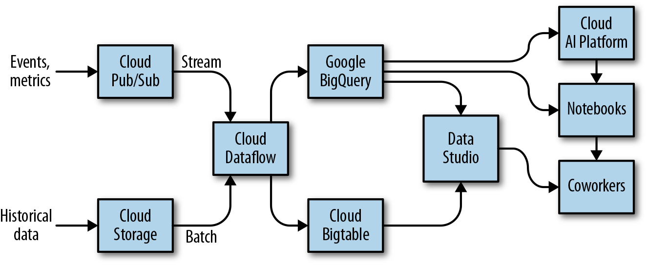
Figure 4-7. Reference architecture for data processing on Google Cloud Platform

In the previous section, we set up a real-time stream of events into Cloud Pub/Sub that we can aggregate in Cloud Dataflow and write to BigQuery. Data Studio can connect to BigQuery and provide a real-time, interactive dashboard. Let’s get started.

Streaming in Java Dataflow

We used Beam/Dataflow in Python in the previous chapter because it was an ETL pipeline without any performance requirements. When we carried out the time correction of the raw flight data, we were working off files in Cloud Storage in batch mode, processing them in Cloud Dataflow and writing events table into BigQuery. Here, though, we need to process events in Cloud Pub/Sub that are streaming in and I anticipate that we will need to use this code in production where there will be strict processing time budgets. While the Python API for Apache Beam is becoming more and more capable, the Java API is much more mature and performant. Therefore, I will do this chapter’s transformations in Java.¹⁹

We could simply receive the events from Cloud Pub/Sub and directly stream them to BigQuery using just a few lines of code:

String topic = "projects/" + options.getProject() + "/topics/arrived";
pipeline //
   .apply("read", PubsubIO.<String>read().topic(topic)) //
   .apply("to_row", ParDo.of(new DoFn<String, TableRow>() {
       @Override
       public void processElement(ProcessContext c) throws Exception {
           String[] fields = c.element().split(",");
           TableRow row = new TableRow();
           row.set("timestamp", fields[0]);
           …
           c.output(row);
       }} ) //
      .apply("write", 
             BigQueryIO.writeTableRows.to(outputTable)
                .withSchema(schema));

In the preceding code, we subscribe to a topic in Cloud Pub/Sub and begin reading from it. As each message streams in, we convert it to a TableRow in BigQuery and then write it out. Indeed, if this all we need, we can simply use the Google-provided Dataflow template that goes from Pub/Sub to BigQuery²⁰. In any case, we can use the open-source Dataflow template²¹ on GitHub as a starting point.

Windowing a pipeline

Although we could do just a straight data transfer, I’d like to do more. When I populate a real-time dashboard of flight delays, I’d like the information to be aggregated over a reasonable interval—for example, I want a moving average of flight delays and the total number of flights over the past 60 minutes at every airport. So, rather than simply take the input received from Cloud Pub/Sub and stream it out to BigQuery, I’d like to carry out time-windowed analytics on the data as I’m receiving it and write those analytics²² to BigQuery. Cloud Dataflow can help us do this.

Because this is Java, and Java code tends to be verbose, I’ll show you only the key parts of the code and keep the snippets I show conceptually relevant. For the full code, see the GitHub repository for this book.²³ You can execute it by using the run_oncloud.sh script that is included (it relies on the Java build tool Maven and Java 8, so you should have both of these installed).

Creating a Java Dataflow pipeline in Java is conceptually similar to doing so in Python. We specify a project, runner, staging directory, and so on as usual on the command line and pull it into our program as command-line args. The one difference here, because we are no longer working with batch data, is that we turn on streaming mode:

MyOptions options = PipelineOptionsFactory.fromArgs(args).//
                    withValidation().as(MyOptions.class);
options.setStreaming(true);
Pipeline p = Pipeline.create(options);

The class MyOptions simply defines two extra command-line parameters: the averaging interval (60 minutes is what I will use in my charts in this section) and the speed-up factor. Because we are simulating real-time, aggregation of 60 minutes of data translates to an actual aggregation of over 1 minute of the incoming stream if we are simulating at 60x. The program uses the desired averaging interval and the speed-up factor to calculate this:

Duration averagingInterval = Duration.millis(Math.round(
      1000 * 60 * (options.getAveragingInterval() / 
                   options.getSpeedupFactor())));

While we may be averaging over 60 minutes, how often should we compute this 60-minute average? It might be advantageous, for example, to use a sliding window and compute this 60-minute average every minute. In my case, I’ll use an averaging frequency that ends up computing the moving average twice²⁴ within the averaging interval, i.e. once every 30 minutes:

Duration averagingFrequency = averagingInterval.dividedBy(2);

Streaming aggregation

The difference between batch aggregation and streaming aggregation starts with the source of our data. Rather than read messages from Cloud Storage, we now read messages from the Cloud Pub/Sub topic. However, what does the “max” mean when the data is unbounded?

A key concept when aggregating streaming data is that of a window that becomes the scope for all aggregations. Here, we immediately apply a time-based sliding window on the pipeline. From now on, all grouping, aggregation, and so on is within that time window:

PCollection<Flight> flights = p //
   .apply(event + ":read", PubsubIO.<String>read().topic(topic))
   .apply(event + ":window", Window.into(SlidingWindows
        .of(averagingInterval).every(averagingFrequency)))

We then convert every message that we read into a Flight object:

.apply(event + ":parse", ParDo.of(new DoFn<String, Flight>() {
@Override
public void processElement(ProcessContext c) throws Exception {
    try {
        String line = c.element();
        Flight f = new Flight(line.split(","), eventType);
        c.output(f);
    } catch (NumberFormatException e) {
        // ignore errors about empty delay fields ...
    }
}
}));

The variable flights is a PCollection (a distributed, out-of-memory collection) that can then be passed on to new parts of the pipeline. Because no group-by has happened yet, flights is not yet subject to a time window.

The Flight object itself consists of the data corresponding to the event. For example, if the eventType is arrived, the airport information corresponds to the destination airport, whereas if the eventType is departed, the airport information corresponds to the origin airport:²⁵

public class Flight implements Serializable {
    Airport airport;
    double delay;
    String timestamp;
}

The Airport information consists of the name of the airport and its geographic coordinates:

public class Airport implements Serializable {
    String name;
    double latitude;
    double longitude;
}

The first statistic that we want to compute is the average delay at any airport over the past hour. We can do this very simply:

stats.delay = flights
   .apply(event + ":airportdelay", \
   ParDo.of(new DoFn<Flight, KV<Airport, Double>>() {
    @Override
    public void processElement(ProcessContext c) throws Exception {
        Flight stats = c.element();
        c.output(KV.of(stats.airport, stats.delay));
    }
   }))//
   .apply(event + ":avgdelay", Mean.perKey());

Ignoring the Java boilerplate introduced by anonymous classes and type safety, this boils down to emitting the delay value for every airport, and then computing the mean delay per airport. Cloud Dataflow takes care of windowing this computation so that the mean happens over the past 60 minutes and is computed every 30 minutes. The result, stat.delay, is also a PCollection that consists of a value for every airport. If we call the method movingAverage() that we looked at earlier, we need to calculate movingAverage() starting from the pipeline twice, once for departed events, and again for arrived events:

final WindowStats arr = movingAverageOf(options, p, "arrived");
final WindowStats dep = movingAverageOf(options, p, "departed");

We want to compute more than just the average delay, however. We want to know how many flights the airport in question handled (perhaps the number of flights at an airport is a predictor of delays) and the last timestamp of the last flight in the window. These two statistics are computed as follows (I’m omitting the boilerplate):

stats.timestamp = flights //
   .apply(event + ":timestamps", …
         c.output(KV.of(stats.airport, stats.timestamp));
      )//
    .apply(event + ":lastTimeStamp", Max.perKey());
for the latest timestamp and:
stats.num_flights = flights //
    .apply(event + ":numflights", ...
         c.output(KV.of(stats.airport, 1));
              )//
    .apply(event + ":total", Sum.integersPerKey());
for the total number of flights.

Co-join by key

At this point, we have six statistics for each airport—the mean departure delay, the mean arrival delay, the latest departure timestamp, the latest arrival timestamp, the total number of departures, and the total number of arrivals. However, they are all in separate PCollections. Because these PCollections all have a common key (the airport), we can “co-join” these to get all the statistics in one place:²⁶

KeyedPCollectionTuple //
.of(tag0, arr_delay) // PCollection
.and(tag1, dep_delay) //
.and(tag2, arr_timestamp) //
// etc.
.apply("airport:cogroup", CoGroupByKey.<Airport> create()) //
.apply("airport:stats", ParDo.of(...
     public void processElement(ProcessContext c) throws Exception {
          KV<Airport, CoGbkResult> e = c.element();
          Airport airport = e.getKey();
          Double arrDelay = e.getValue().getOnly(tag0,
                                         new Double(-999));

          // etc.
          c.output(new AirportStats(airport, arrDelay, depDelay,
                                    timestamp, num_flights));
}}))//

The class AirportStats contains all the statistics that we have collected:

public class AirportStats implements Serializable {
     Airport airport;
     double arr_delay, dep_delay;
     String timestamp;
     int num_flights;
}

These can be written to BigQuery with a schema, as discussed in the section on simulating a real-time feed.

Executing the Stream Processing

To start the simulation, start the Python simulator that we developed in the previous section:

python simulate.py --startTime '2015-05-01 00:00:00 UTC' 
--endTime '2015-05-04 00:00:00 UTC'  --speedFactor 30

The simulator will send events from May 1, 2015, to May 3, 2015, at 30 times real-time speed, so that an hour of data is sent to Cloud Pub/Sub in two minutes. You can do this from CloudShell or from your local laptop. (If necessary, run install_packages.sh to install the necessary Python packages and gcloud auth application-default login to give the application the necessary credentials to execute queries.)

Then, start the Cloud Dataflow job that will listen to the two Cloud Pub/Sub topics and stream aggregate statistics into BigQuery. You can start the Cloud Dataflow job using Apache Maven:

mvn compile exec:java \
 -Dexec.mainClass=com.google.cloud.training.flights.AverageDelayPipeline
      -Dexec.args="--project=$PROJECT \
      --stagingLocation=gs://$BUCKET/staging/ \
      --averagingInterval=60 \
      --speedupFactor=30 \
      --runner=DataflowRunner"

If you now browse to the Cloud Platform console, to the Cloud Dataflow section, you will see that a new streaming job has started and that the pipeline looks like that shown in Figure 4-8.

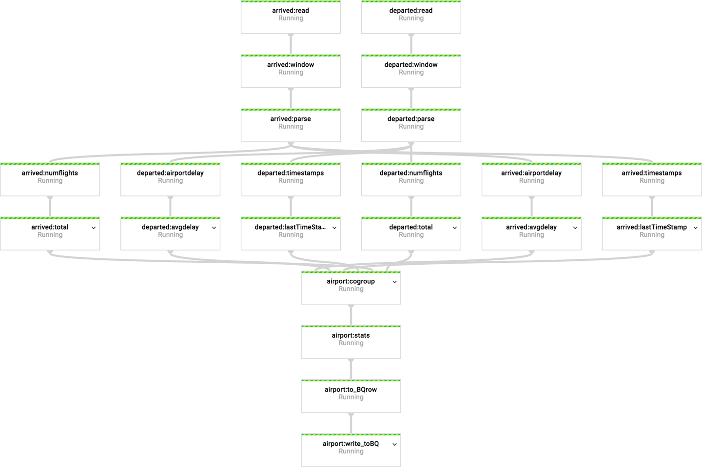
Figure 4-8. The streaming pipeline to compute three sets of statistics

From each of the topics, three sets of statistics are computed, cogrouped into a single AirportStats object and streamed into BigQuery.

Analyzing Streaming Data in BigQuery

Three minutes²⁷ after the launch of your program, the first set of data will make it into BigQuery. You can query for the statistics for a specific airport from the BigQuery console:

#standardsql
SELECT
  *
FROM
  `flights.streaming_delays`
WHERE
  airport = 'DEN'
ORDER BY
  timestamp DESC

Figure 4-9 presents the results that I got.

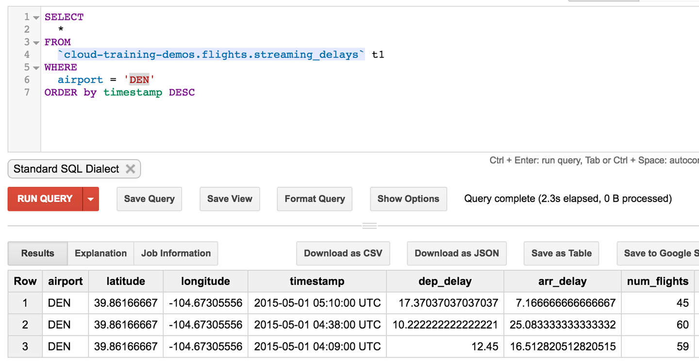
Figure 4-9. Results of the streaming pipeline shown for Denver airport

Note how the timestamps are spread about 30 minutes apart. The average delays themselves are averages over an hour. So, Denver airport in the time between 04:10 UTC and 05:10 UTC had 45 flights, and an average departure delay of 17 minutes.

The cool thing is that we can do this querying even as the data is streaming! How would we get the latest data for all airports? We could use an inner query to find the maximum timestamp and use it in the WHERE clause to select flights within the past 30 minutes:

#standardsql
SELECT
  airport,
  arr_delay,
  dep_delay,
  timestamp,
  latitude,
  longitude,
  num_flights
FROM
  flights.streaming_delays
WHERE
  ABS(TIMESTAMP_DIFF(timestamp,
      (
      SELECT
        MAX(timestamp) latest
      FROM
        `cloud-training-demos.flights.streaming_delays` ),
      MINUTE)) < 29
  AND num_flights > 10

Figure 4-10 shows the results.

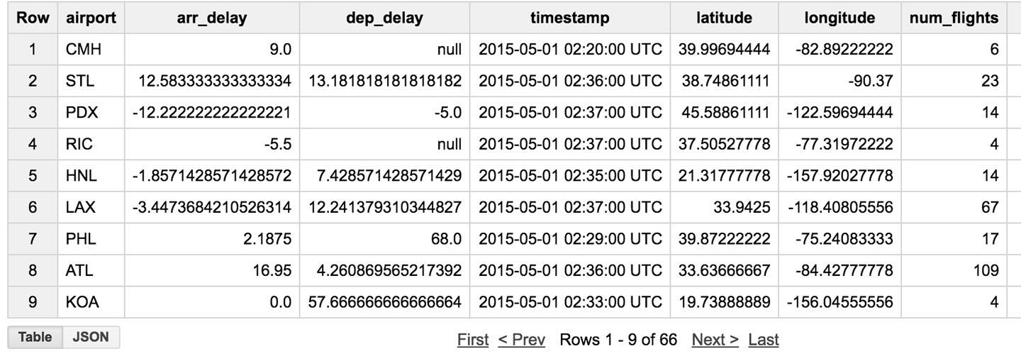
Figure 4-10. The latest results for all airports

Queries like these on streaming data will be useful when we begin to build our dashboard. For example, the first query will allow us to build a time–series chart of delays at a specific airport. The second query will allow us to build a map of average delays across the country.

Real-Time Dashboard

Now that we have streaming data in BigQuery and a way to analyze it as it is streaming in, we can create a dashboard that shows departure and arrival delays in context. Two maps can help explain our contingency table–based model to end users: current arrival delays across the country, and current departure delays across the country.

To pull the data to populate these charts, we need to add a BigQuery data source in Data Studio. Although Data Studio supports specifying the query directly in the user interface, it is much better to create a view in BigQuery and use that view as a data source in Data Studio. BigQuery views have a few advantages over queries that you type into Data Studio: they tend to be reusable across reports and visualization tools, there is only one place to change if an error is detected, and BigQuery views map better to access privileges (Cloud Identity Access Management roles) based on the columns they need to access.

Here is the query that I used to create the view:

#standardSQL
SELECT
  airport,
  last[safe_OFFSET(0)].*,
  CONCAT(CAST(last[safe_OFFSET(0)].latitude AS STRING), ",", 
        CAST(last[safe_OFFSET(0)].longitude AS STRING)) AS location
FROM (
  SELECT
    airport,
    ARRAY_AGG(STRUCT(arr_delay,
        dep_delay,
        timestamp,
        latitude,
        longitude,
        num_flights)
    ORDER BY
      timestamp DESC
    LIMIT
      1) last
  FROM
    flights.streaming_delays
  GROUP BY
    airport )

This is slightly different from the second query in the previous section (the one with the inner query on maximum timestamp). It retains the last received update from each airport, thus accommodating airports with very few flights and airports with which we have lost connectivity over the past hour (in practice, you’d add filtering to this query to avoid displaying data that is too old). The query also combines the latitude and longitude columns into a single text field that is separated by a comma. This is one of the geographic formats understood by Data Studio.

Figure 4-11 presents the end result.

Having saved the view in BigQuery, we can create a data source for the view in Data Studio, very similar to the way we created one for views in Cloud SQL in the previous chapter. Make sure to change the type of the location column from Text to Geo → Latitude, Longitude.

Figure 4-11. Result of query to get latest data from all airports, along with location information

After the data source has been created, you are ready to create a geo map (using the globe icon in Data Studio). Change the zoom area to the United States, specify dep_delay as the metric, and change the style so that the color bar goes from green to red through white. Repeat this for the arrival delay and the total number of flights, and you’ll end up with a dashboard that looks like the one shown in Figure 4-12.

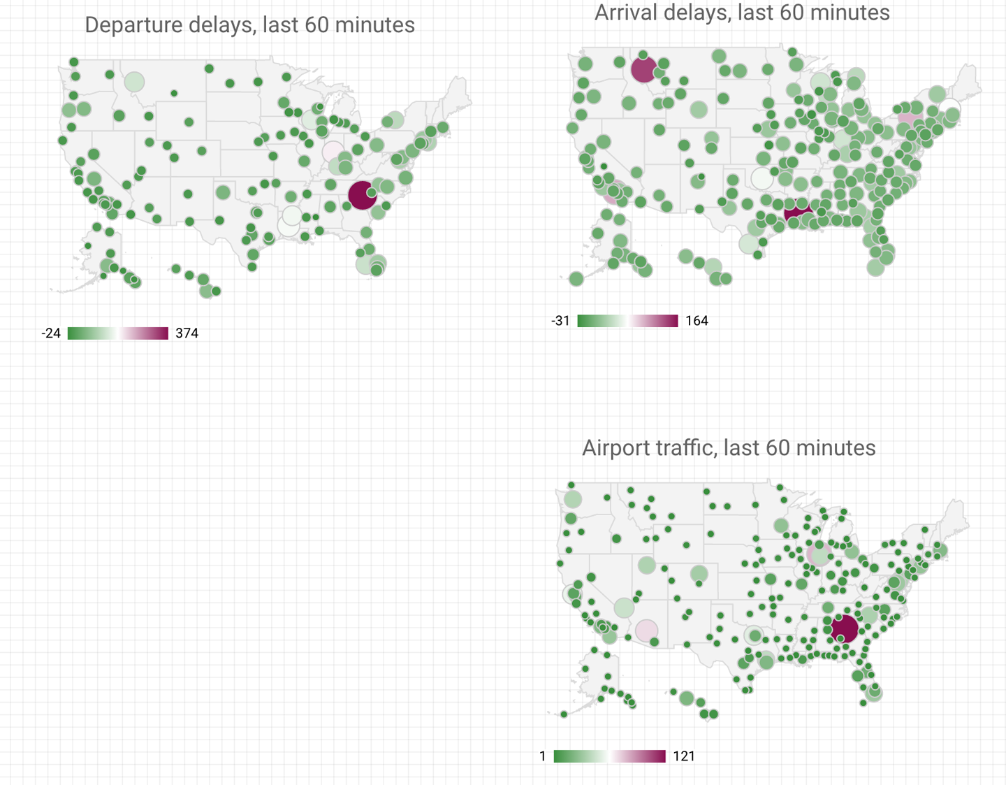
Figure 4-12. Dashboard of latest flight data from across the United States

It is worth reflecting on what we did in this section. We processed streaming data in Cloud Dataflow, creating 60-minute moving averages that we streamed into BigQuery. We then created a view in BigQuery that would show the latest data for each airport, even as it was streaming in. We connected that to a dashboard in Data Studio. Every time the dashboard is refreshed, it pulls new data from the view, which in turn dynamically reflects the latest data in BigQuery.

Summary

In this chapter, we discussed how to build a real-time analysis pipeline to carry out streaming analytics and populate real-time dashboards. In this book, we are using a dataset that is not available in real time. Therefore, we simulated the creation of a real-time feed so that I could demonstrate how to build a streaming ingest pipeline. Building the simulation also gives us a handy test tool—no longer do we need to wait for an interesting event to happen. We can simply play back a recorded event!

In the process of building out the simulation, we realized that time handling in the original dataset was problematic. Therefore, we improved the handling of time in the original data and created a new dataset with UTC timestamps and local offsets. This is the dataset that we will use going forward.

We also looked at the reference architecture for handling streaming data in Google Cloud Platform. First, receive your data in Cloud Pub/Sub so that the messages can be received asynchronously. Process the Cloud Pub/Sub messages in Cloud Dataflow, computing aggregations on the data as needed, and stream either the raw data or aggregate data (or both) to BigQuery. We worked with all three Google Cloud Platform products (Cloud Pub/Sub, Cloud Dataflow, and BigQuery) using the Google Cloud Platform client libraries in Python. However, in none of these cases did we ever need to create a virtual machine ourselves—these are all serverless and autoscaled offerings. We thus were able to concentrate on writing code, letting the platform manage the rest.

¹ Note that this is a common situation. It is only as you start to explore a dataset that you discover you need ancillary datasets. Had I known beforehand, I would ingested both datasets. But you are following my workflow, and as of this point, I knew that I needed a dataset of timezone offsets but hadn’t yet searched for it!

² For example, the time zone of Sevastopol changed in 2014 from Eastern European Time (UTC+2) to Moscow Time (UTC+4) after the annexation of Crimea by the Russian Federation.

³ For example, is there a spike associated with traffic between 5 PM and 6 PM local time?

⁴ The Java API is much more mature and performant, but Python is easier and more concise. In this book, we will use both.

⁵ See http://data-artisans.com/why-apache-beam/ and https://github.com/apache/incubator-beam/tree/master/runners/flink.

⁶ This code is in 04_streaming/simulate/df01.py of the GitHub repository of this book. Before you run it, you might have to install Apache Beam. You can do that using the install_packages.sh script in the repository.

⁷ This code is in 04_streaming/simulate/df02.py of the GitHub repository of this book.

⁸ See the answer to the question “How do I handle NameErrors?” at https://cloud.google.com/dataflow/faq.

⁹ If you are running this in CloudShell, find the button on the top right that allows you to “boost” the virtual machine. You will have to reinstall the packages using the install_packages.sh script.

¹⁰ This code is in 04_streaming/simulate/df03.py of the GitHub repository of this book.

¹¹ This code is in 04_streaming/simulate/df04.py of the GitHub repository of this book.

¹² This code is in 04_streaming/simulate/df05.py of the GitHub repository of this book.

¹³ Code for this section is in 04_streaming/simulate/df06.py of the GitHub repository of this book.

¹⁴ It might be better to create the table outside of the pipeline if you want to partition it by date, for example.

¹⁵ The file 04_streaming/simulate/df06.py of the GitHub repository of this book.

¹⁶ The code for this is in simulate.py in 04_streaming/simulate in the GitHub repository for this book.

¹⁷ Also, when the script runs out of records to process, it will essentially just time out with an error. If that happens, restart the script.

¹⁸ For an example, go to https://cloud.google.com/solutions/mobile/mobile-gaming-analysis-telemetry.

¹⁹ My treatment of Beam Java syntax in this section is going to be quite rapid; mostly, I focus on streaming data concepts. In Chapter 8, where Beam Java makes a reappearance, I spend more time on the syntactic details. Come back and reread this section after you read Chapter 8.

²⁰ See https://cloud.google.com/dataflow/docs/guides/templates/provided-streaming#cloudpubsubtobigquery

²¹ See https://github.com/GoogleCloudPlatform/DataflowTemplates/blob/master/src/main/java/com/google/cloud/teleport/templates/PubSubToBigQuery.java

²² If you wanted to write the raw data that is received to BigQuery, you could do that, too, of course—that is what is shown in the previous code snippet. In this section, I assume that we need only the aggregate statistics over the past hour.

²³ See the Java code in 04_streaming/realtime/chapter4/src of http://github.com/GoogleCloudPlatform/data-science-on-gcp.

²⁴ Computing a moving average will end up causing loss of information, of course, but given that we are going to be computing a moving average, doing so at least twice within the window helps preserve the information whose variation can be captured by that window. This result, proved by Claude Shannon in 1948, launched information theory as a discipline.

²⁵ Because the Flight object is Serializable, Java serialization will be used to move the objects around. For better performance, we should consider using a protocol buffer. This pipeline is not going to be used routinely, and so I will take the simpler route of using Java serialization in this chapter. When we do real-time serialization in later chapters, we will revisit this decision.

²⁶ The code shown here is greatly simplified. For the full code, see the GitHub repository.

²⁷ Recall that we are computing aggregates over 60 minutes every 30 minutes. Cloud Dataflow treats the first “full” window as happening 90 minutes into the simulation. Because we are simulating at 30 times speed, this is three minutes on your clock.