Digital Filters Design for Signal and Image Processing

8.4. Filtering in the spatial domain

A filtering operation can be carried out by discrete convolution, which is the digital version of equation (8.4). When 2-D signals represent images of the real world, they are modelized by non-stationary random fields, which can be considered as being locally stationary. Here, optimal operators turn out to be non-stationary operators as well. Implementation techniques consist of locally adapting the coefficients of a linear filter. This is the reason why their characteristics are introduced here.

8.4.1. 2-D discrete convolution

Let s be the input signal and w the output signal. The input/output relationship is given by a discrete convolution equation:

where h(k,l) denotes the impulse response of the 2-D filter.

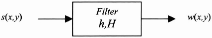
Figure 8.8. 2-D discrete linear filtering

The filter can be implemented using equation (8.16) when the number of non-null coefficients of the impulse response is finite.

At each pixel, the inner product of the “coefficients” vector by the “data” vector has to be calculated. For an impulse response of M × N coefficients, the number of multiplications by pixel is MN. When the 2-D signal represents an image, odd dimensions are generally chosen in order to symmetrize the processing around the current pixel.

Figure 8.9. Implementation of a ...