Excel 2007 Pocket Guide, 2nd Edition

Chapter 1. Understanding Excel

The first chapter of this book is designed to give those readers with relatively little experience using Excel 2007 enough information to dive right in and start creating rich Excel workbooks immediately, and to fill in some of the details for more experienced Excel users who haven’t had enough time to examine the program and its new user interface in depth.

This chapter covers:

• What’s new in Excel 2007

• The Excel interface

• Workbook, template, and workspace files

• The anatomy of an Excel file

• Formatting

• Shortcut Menus and the Mini Toolbar (a.k.a. the “floatie”)

What’s New in Excel 2007

After the significant leap forward from Excel 95 to Excel 97, Excel versions 2000, 2002, and 2003 were incremental improvements on the same basic application design. By contrast, Excel 2007 is a substantial departure from Excel 2003. Excel 2007 comes with a new user interface (detailed later in this chapter), a much larger worksheet, and new formatting capabilities, among many other changes. Table 1-1 summarizes the most important changes in Excel 2007.

Table 1-1. Excel 2007 greatly expands the size of the worksheet and extends the possible number of sorting levels, characters in a cell, and colors in a workbook.

Capability	Old limit	New limit
Worksheet size	65,536 rows by 256 columns	1,048,576 rows by 16,384 columns
Total characters in a cell	1,024 characters	32,767 characters
Total characters printed in a cell	1,024 characters	32,767 characters
Colors in a workbook	56	16 million colors
Undo levels	16	100
Sort levels	3	64
Conditional format conditions	3	Limited by available memory
Maximum length of a formula	1,024 characters	8,192 characters
Maximum number of arguments to a function	30	255
Number of nested levels allowed in a formula	7	64

Note

The new limits only apply when you save a workbook using the new Office 2007 file format. If you save a work-book using the old Excel 97–2003 file format, the old limits apply.

The Excel 2007 Interface

Excel’s interface stayed more or less constant from Excel 97 to Excel 2003. During that time, the program’s developers added some new features and moved items around in the menu and toolbar system, but the basic structure remained the same. All that changed in Office 2007.

The Ribbon

Excel 2007, Word 2007, and PowerPoint 2007 all use the new Microsoft Office Fluent interface design, commonly referred to as the Ribbon (Figure 1-1).

Figure 1-1. The Home tab of the new Excel 2007 user interface Ribbon.

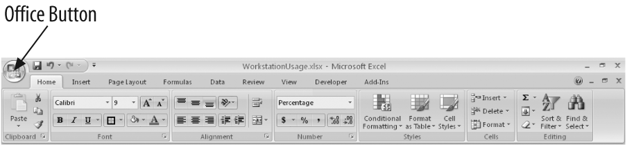
Figure 1-1 shows one tab from the new Ribbon user interface, which replaces the menu bars and toolbars (collectively known as command bars) found in Excel 2003. The Ribbon contains most, but not all, of the commands available in Excel 2007. The Microsoft Office user experience team created the new Ribbon interface in an effort to make it easier to discover the full range of built-in capabilities in Excel 2007. The Office product teams constantly receive requests for features that were already built into the programs, so they designed the new interface and applied it to the three most popular Office programs.

Note

The Ribbon resizes itself and its controls to reflect your monitor’s resolution and the window size, so you might see a different set of controls (and differently appearing controls) than is shown in Figure 1-1.

Rather than force users to poke through a maze of menus, toolbars, and dialog boxes to find the commands they’re looking for, the Ribbon brings most of Excel’s functionality to the top level of the user interface. The Home tab, shown in Figure 1-1, contains the most common operations: cutting and pasting, font and cell formatting, finding and selecting cells, and so on.

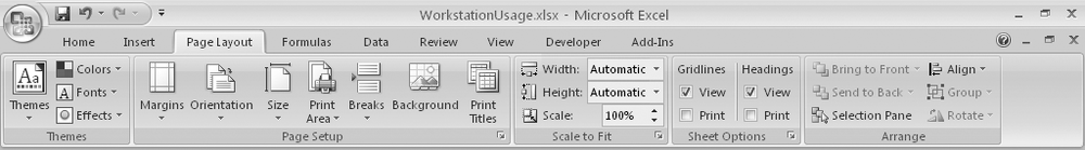
The Page Layout tab of the Ribbon (Figure 1-2) hosts buttons that enable you to change the page’s appearance and control printing. For example, you can change a worksheet’s margins, turn gridlines on and off, select the parts of the worksheet you want to print, and add a background image.

Figure 1-2. The controls on the Page Layout tab let you determine how your page looks when it’s displayed and printed.

Tip

To hide the Ribbon, press Ctrl-F1. Pressing Ctrl-F1 again brings the Ribbon back. When the Ribbon is hidden, clicking on the menu temporarily brings the Ribbon back.

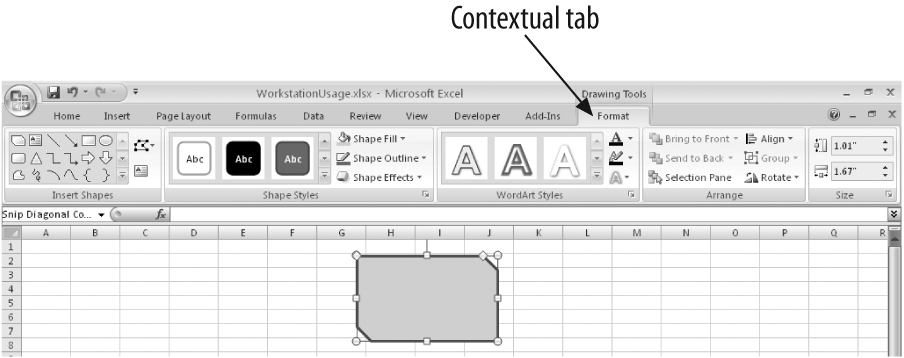
Contextual Tabs

Previous versions of Excel displayed toolbars with buttons and menus you could use to change a selected object, such as an image you inserted into a worksheet. Excel 2007 doesn’t use the command bar user interface, so the designers created contextual tabs (Figure 1-3), which appear on the Ribbon when you select an object with associated controls that don’t appear on the basic Ribbon.

Contextual tabs appear at the right end of the Ribbon and are a different color than the regular Ribbon tabs.

Figure 1-3. Excel 2007 displays contextual tabs when selected objects require controls that don’t appear on the basic Ribbon.

Dialog Expanders

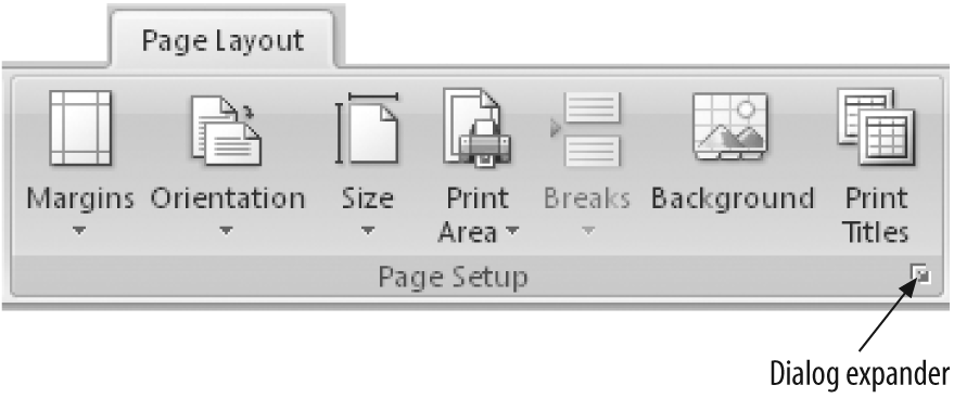
The new Excel 2007 user interface brings the most commonly used controls to the top level of the Ribbon. You’ll still need to display a lot of dialog boxes to make the changes you want, particularly when it comes to page setup tasks such as changing margins. Excel 2007 indicates there’s a dialog box available in two ways. First, if a Ribbon button’s label is followed by three dots, clicking the button displays a dialog box. Second, some Ribbon groups have a dialog expander at the bottom-right corner of the group (see Figure 1-4). Clicking the dialog expander control displays a dialog box related to the group’s controls.

Figure 1-4. When you need finer control over your worksheet, open a dialog box to display the full range of changes you can make to the selected item.

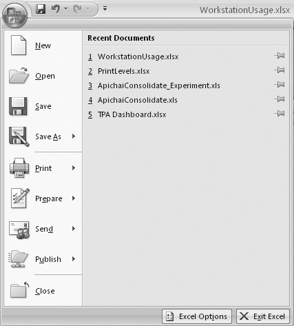
The Office Button

When using Excel 2007 for the first time, many experienced Excel users ask, “Where is the File menu?” Early drafts of the Excel 2007 interface did have a File menu at the top-left corner of the Ribbon, but the Office user interface design team removed the File menu and replaced it with the Microsoft Office Button (Figure 1-5).

Figure 1-5. You can find the familiar File menu items, such as Save, Save As, Print, and Close by clicking the Microsoft Office Button.

Note

If you provide technical support to your colleagues who use Excel 2007, you should consider sending them all an email message indicating that they can find the File menu functions by clicking the Office Button. The one minute you spend composing that message will save you hours of tech support calls.

Quick Access Toolbar

Just to the right of the Office Button, you’ll find the Quick Access Toolbar. The Quick Access Toolbar contains three buttons by default: the Save button, the Undo button (for undoing changes you just made), and the Redo/Repeat button (which lets you reverse a click of the Undo button or, depending on what you just did, repeat an operation).

You can add any Ribbon button or group to the Quick Access Toolbar by right-clicking the button or group’s name and selecting the “Add to Quick Access Toolbar” menu item.

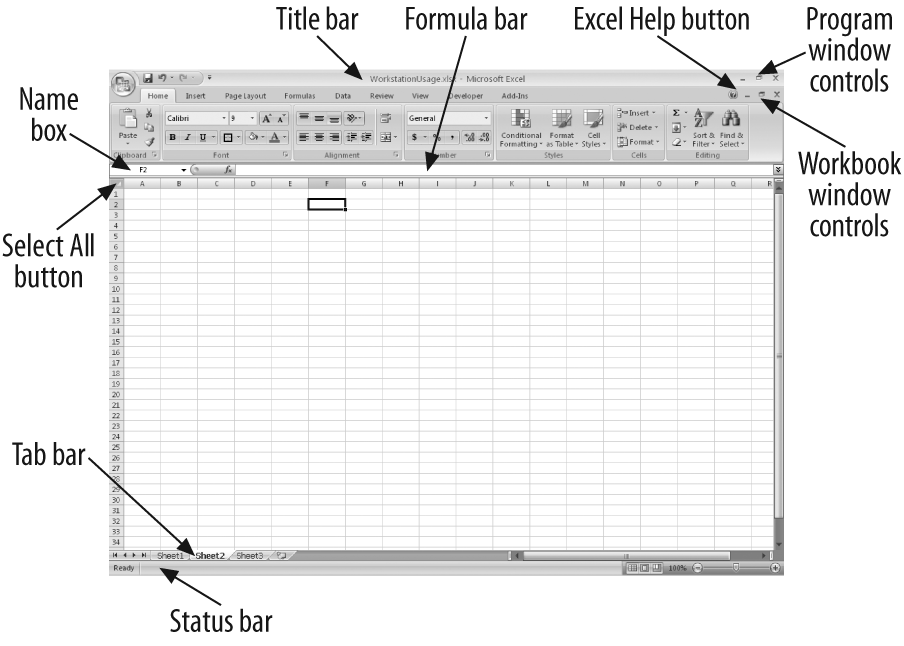
The Excel Program Window

Aside from the Ribbon, the Excel 2007 user interface has changed little from Excel 97. Figure 1-6 shows the Excel 2007 program window; the text that follows describes the elements you’ll use the most.

Title bar

The title bar, which appears at the top of the Excel window, shows the name of the workbook and any file access restrictions. If you display the Open dialog box and click the down arrow at the right edge of the Open button, you can open a selected workbook as a copy of the original in read-only mode, in repair mode, or (if the file is web-compatible) in a browser. Whichever status you select will be displayed on the title bar.

Figure 1-6. The Excel 2007 user interface.

Excel Help button

The Excel Help button, which is a round blue button with a white question mark in the center, appears near the top-right corner of the Excel program window. Clicking the Excel Help button displays the Excel Help window, which contains links to popular topics and a search box where you can type words and phrases you’d like to look up.

Formula bar

The formula bar displays the content of the active cell or the formula that generated that content. You edit the contents of a cell by clicking in the formula bar and using the mouse and keyboard. You can also double-click the cell and edit in it directly. (After you type the function and the opening parentheses, for example =SUM(, the program displays information about what kind of input the formula you are entering requires—e.g., the SUM formula expects one or more cell ranges.)

Name box

The name box displays the reference of the active cell (e.g., B2) or displays the size of a selected group of cells (e.g., 2R x1C, or “two rows by one column”). When the mouse button is released, a reference to the first cell selected appears in the box. The name box also lists the named ranges in the worksheet. Open the name box and select a named range to highlight the cells in that range.

Tip

You can get more information on named ranges in Chapter 2 under the section “Using Named Ranges.”

Program window controls

At the top right of the Excel window are four controls: the Minimize button, which reduces the Excel program window to a button on the task bar; the Restore button, which toggles the program window between smaller and larger sizes; the Maximize button, which appears when the program window is reduced in size; and the Close button, which exits Excel.

Workbook window controls

Just below the program window controls are a similar set of controls for each open workbook. Click a workbook’s Minimize button and it becomes a title bar within the larger Excel window; click the Restore button to toggle the workbook between smaller and larger sizes; click the Maximize button to expand the workbook to fill the window; and click Close to close the workbook.

Select All button

Clicking the Select All button, located at the top-left corner of a worksheet (to the left of the Column A header and above the Row 1 header), selects every cell in a worksheet. Pressing Ctrl-A does the same thing.

Tab bar

Every worksheet in a workbook is represented (at the bottom of the window) by a tab. Clicking a tab displays the corresponding worksheet, while right-clicking a tab displays a shortcut menu with options to insert a new worksheet; rename, delete, or move the selected worksheet; select all the worksheets; or access VBA code for that sheet. You can change a worksheet tab’s color if you want to make it stand out from the other worksheets.

Status bar

The Excel status bar (Figure 1-7) displays the current state of the program; lists any background tasks that are running, such as saves; and displays a running summary of numerical values in currently selected cells. You can change the summary operations or turn them off.

Figure 1-7. The Excel status bar, showing the sum, average, and count of selected cells in the worksheet.

New Excel 2007 File Format

One of the most significant changes between Office 2003 and Office 2007 is that the three most popular programs (Word, Excel, and PowerPoint) use a new file format that is substantially different from the format used in Excel 97–2003. The new file format, which is based on the Extensible Markup Language (XML), separates Excel 2007 workbooks into different components—creating text files where possible—and uses the ZIP compression algorithm to reduce the file’s size.

Separating a workbook’s worksheets, charts, drawings, printer settings, and tables into different files reduces the likelihood that a hard disk failure will ruin an entire Excel 2007 workbook. If Excel can’t open part of the file, it displays an error message but opens as much of the workbook as it can.

Note

If you want to look at an Excel 2007 file’s structure, save a copy of a workbook in a new folder. Then, in Windows Explorer or My Computer, change the file’s extension to .zip (e.g., if the workbook’s name is Dashboard.xlsx, change it to Dashboard.zip). When you double-click the file, Windows XP or Vista will display the file’s components. Double-clicking the XML file you want to display opens the file in Internet Explorer or your web browser of choice.

Even though Excel 97–2003 can’t open Excel 2007 files without downloading and installing additional software, Excel 2007 can open earlier files with no difficulty. When you open an Excel 97–2003 file in Excel 2007, the program opens it in Compatibility Mode, which prevents you from adding new formats, charts, drawings, or other features not present in Excel 2003. If you want to save an Excel 97–2003 file as an Excel 2007 file, which enables the new features, click Office Button → Save As and set the file type to Excel Workbook.

Tip

If you want to open Excel 2007 workbooks in Excel 2002 or 2003, install the Microsoft Office Compatibility Pack. You can find instructions for downloading and installing the Compatibility Pack on the Microsoft web site at http://support.microsoft.com/kb/923505. You can also go to http://msdn.microsoft.com and search “Office Compatibility Pack.”

Workbook, Template, and Workspace Files

Excel 2007 uses six primary file types:

• A workbook file (.xlsx) contains individual worksheets, which can contain cell values, formulas, formatting information, styles, graphics, drawing objects, hyperlinks, charts, and data validation settings. Files saved using the default .xlsx format cannot contain macros. You can open and edit files in other formats, such as text files (.txt), Excel files created using previous program versions (.xls), and Access database tables, but those files will not have all of the built-in functionality that comes with Excel. You can, of course, save Excel workbooks in any of the aforementioned formats—and more.

  Note

  Excel 97–2003 could open Lotus 1-2-3 files, but Excel 2007 no longer supports files created using that program.

• A macro-enabled workbook (.xlsm) file is the same as a standard workbook (.xlsx) file, except that it enables you to record macros that you can replay to repeat a procedure without going through the individual steps again. Excel records its macros in the Visual Basic for Applications (VBA) programming language, which lets programmers make changes to the computers where the macro file resides. Evildoers write viruses and other harmful programs using VBA, so Microsoft changed the Excel 2007 file formats and macro security settings to help prevent malicious software from infecting your computer. Excel 2007 will only run macros if they are contained in a workbook of the proper type (.xlsm or .xls), and you give Excel permission to run the macro.

• A template (.xltx) file holds all of the information that a standard workbook file contains, plus styles formatting and other settings that have been applied. For example, if you create a workbook to record monthly expenses in three categories, you can lay out all the elements and save it as a template. When you base a new file on a template, you get the headings, instructions, formatting, and so on that you created previously—a blank boilerplate that can now hold fresh data. (Just remember to save your work as an .xlsx file.)

• Just as template (.xltx) files enable you to create standard (.xlsx) workbooks, macro-enabled templates (.xltm) let you create identical copies of macro-enabled workbooks (.xlsm).

• A workspace file (.xlw) contains pointers to other Excel files that you had open during a session. When you open a workspace file, Excel opens all the other Excel files it refers to. Workspace files are particularly useful if you frequently work with the same set of files and need to have them all open at once.

• If the AutoRecover feature is on (Office Button → Excel Options), click the Save category, and check the "Save AutoRecover info every x minutes” box. Excel creates a quick backup of your work periodically. AutoRecover will often get most, if not all, of your data back in the event of a crash, but it’s no substitute for clicking the Save button frequently. You can find where each version of Excel saves its AutoRecover files, along with other default file locations, in Chapter 3.

Tip

The best time to save a workbook is after you have done something you would hate to have to do again, which means that clicking the Save button should become a reflex. Don’t rely on AutoRecover to save your work for you!

Tips on Using Templates

• Always save your templates in the default Excel template folder. If you installed Office 2007 on your C: drive and didn’t change any folder settings, that folder is C:\Documents and Settings\username\Application Data\ Microsoft\Templates. In that directory path, the string username represents the name of the Windows account you’re currently using. Saving templates in that folder causes the templates to appear in the New Workbook dialog box when you click Office Button → New, and then click the My Templates category header.

• When you create a workbook from a template, you create a new workbook based on the template. However, if you use the Open dialog box to open the template file, you will be editing the template.

• Right-click a template, click New, and you will create a new workbook based on the template.

• To create a template for a worksheet, delete all but one worksheet in a workbook, apply the desired settings (formats, styles, repeating rows and columns, etc.), and save the workbook as a template (.xltx file for normal workbooks or .xltm file for macro-enabled workbooks).

• The templates available in the Spreadsheet Solutions section of the Templates dialog box are formatted for common business uses, such as time cards, balance sheets, expense reports, purchase orders, and sales invoices. (To display the templates, click Office Button → New, and click the Installed Templates category heading.)

Tip

If you click Office Button → New and click the Installed Templates category header, Excel displays the same templates you’ll see if you were to right-click a sheet tab, click Insert, and click the Spreadsheet Solutions tab. The difference between the two operations is that the former procedure creates a new workbook, while the latter adds the template’s worksheets to your existing workbook.

The Anatomy of an Excel File

Think of an Excel file as a collection of data about a given topic, such as sales revenue or time spent on projects. For example, if you were keeping track of your billable hours on a series of projects and had to submit your hours each week, you could create a workbook representing a year and use each worksheet to record your hours per week. You would need to add worksheets for each week (a workbook’s default is three), but the grouping would make sense. If your company maintained a quarterly billing cycle, you could also keep your hours in workbooks of only 13 worksheets, each representing a week in a fiscal quarter.

A Workbook

While an Excel workbook appears to be a single entity, there are actually three different layers: the data layer (the ground floor of your document that holds the worksheet data, formulas, and so on); a back drawing layer (the basement, where you can put background images, such as wallpaper or different colors that make the data easier to read); and a top drawing layer (the second floor, where you can add graphics to highlight important data, or display comments in a text box). Figure 1-8 illustrates how the three layers interact within a workbook.

Figure 1-8. This worksheet has elements in the back drawing layer, data layer, and top drawing layer.

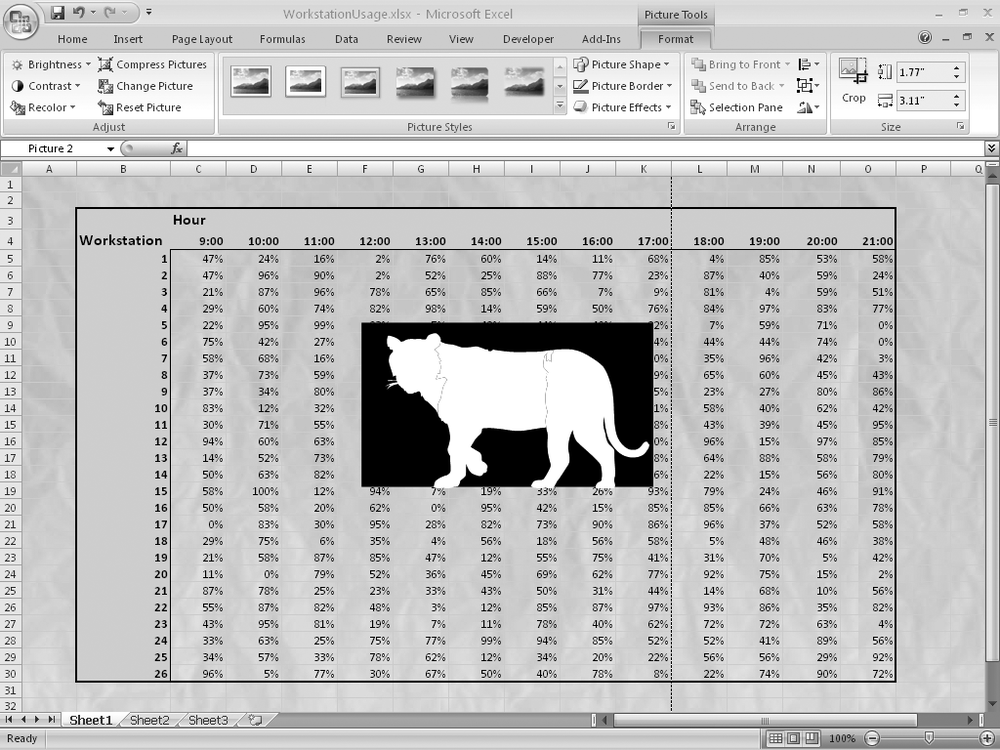
The lines in the background of the sheet are repetitions of a texture graphic, while the image of a tiger is a clip art file. The contents on a higher drawing layer obscure the contents of a lower layer. In Figure 1-8, the picture of the tiger obscures data contained in the worksheet’s cells; in turn, the cell data obscures the background pattern.

A Worksheet

In Excel, worksheets are where the rubber meets the road; worksheets hold your data, formulas, images, and formatting. Worksheets are tables made up of columns and rows—you can identify a cell in an Excel worksheet based on its column (which are lettered) and its row (which are numbered, e.g., A5).

Tip

If you would rather refer to a cell’s address only by numbers, use “R1C1” notation, where the row is preceded by the letter “R”, and the column is preceded by the letter “C”. R1C1 refers to cell A1, R2C2 to cell B2, and so on.

To see your formulas in R1C1 reference format, click Office Button → Excel Options, click the Formulas category header, and check the R1C1 Reference Style box.

Sheet Tabs

The sheet tabs, found on the tab bar at the lower left of the Excel window (Figure 1-9), don’t get a lot of attention. But the sheet tabs (and the tab bar) are useful for organizing and customizing your workbooks. You can change the order of the worksheets by dragging a worksheet tab to the desired spot. Right-click a sheet tab and from the shortcut menu you can rename the worksheet and change other attributes.

Figure 1-9. The tab bar lets you manage the worksheets in your workbook.

You can change the color of a sheet tab, which makes it easy to identify individual worksheets, such as a worksheet where you changed some values. It’s also a handy organizational tool—you could, for example, color code tabs by fiscal quarter.

Tip

A lot of people concentrate on organizing data within a worksheet and forget how the worksheets fit within the workbook as a whole. Use the sheet tabs and the tab bar to organize data by category.

Formatting

The data and formulas that fill a workbook are, ultimately, the most important part of your work with Excel, but how you present your data can make the difference between an easily understood summary and a difficult slog through a twisty maze of numbers. Each workbook element has formatting characteristics that you can change to maximize the effectiveness of your information.

Worksheets

Compared to the other elements of a workbook, there are very few formatting options you can apply to a worksheet as a whole. You can change the margins (Page Layout → Margins), or add a header and footer to a worksheet. As shown in Figure 1-10, a header is a block of space reserved at the top of a page, while a footer is a block of space reserved at the bottom of a page. The text in a header and footer—the date, your company name, etc.—repeats on every printed page of the worksheet they’re attached to. To display the “Header and Footer” dialog box, click Insert → Header and Footer, add custom text, or include AutoText entries such as the time, date, page number, and total number of pages for the worksheet. You can also include images in a header or footer.

Figure 1-10. A header and footer repeat information, such as page numbers and dates, on each printed page.

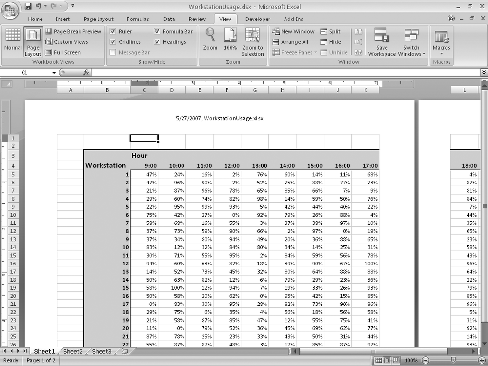
In a similar vein, you can repeat column and row titles on subsequent pages. Click the Page Layout tab, click the Page Setup group’s dialog expander, and then click Sheet to display the Sheet tab of the Page Setup dialog box. Using the “Rows to Repeat at Top” and “Columns to Repeat at Left” controls, you can select the titles you want to appear on each page. If you’re printing a worksheet that requires two or more pages, strongly consider repeating the row and column headers on each page.

Just remember that setting rows and columns to repeat on each printed page doesn’t help as you scroll through a worksheet. Scroll far enough and those headings will disappear. You can freeze rows and columns so they remain visible as you scroll through a worksheet by clicking the cell below and to the right of the rows and columns you want to remain constant, clicking View → Freeze Panes, and selecting whether to freeze rows and columns based on the current selection, freeze just the first row, or freeze just the first column. You can return your worksheet to normal by clicking View → Freeze Panes → Unfreeze Panes.

Tip

Freezing panes has no effect on how the worksheet is printed. Using the controls on the Sheet page of the Page Setup dialog box has no impact on your worksheet as you view it in the Excel window.

One of the toughest decisions when formatting a worksheet’s contents is to determine the appearance of each element. Data labels, headings, and the data itself must be formatted. There is a lot to keep track of, but Excel 2007 comes with a wide array of Office Themes you can apply to your workbooks. To see how an Office Theme affects your worksheet’s appearance, click Page Layout → Themes, and then hover your mouse pointer over the theme you’d like to apply. Even if there isn’t an Office Theme to your liking, you can change the colors, fonts, and text effects in an existing theme and save it as a new theme for later use.

Finally, if you want to hide one or more worksheets in your workbook, simply click its tab, then click Home → Format → Hide & Unhide → Hide Sheet. To unhide it, click Home → Format → Hide & Unhide → Unhide Sheet, and select the worksheet to reveal from the Unhide dialog box. Hiding a worksheet is not a good way to secure its contents, but it’s an easy way to direct attention to the worksheets you want your colleagues to notice.

Columns and Rows

The highest level of organization within a worksheet is the column and the row. Columns are vertical collections of cells, and each column is designated by a letter. Rows are horizontal and are designated by a number. The standard column is 56 pixels wide, and the standard row is 16 pixels high—tall and wide enough to hold a little over eight characters in the default 9-point Calibri font.

Tip

A pixel is a dot on your computer screen, so the amount of space a row or column takes up on your screen depends on the size and resolution of your monitor.

You can change the height of a row or the width of a column by dragging a border of the row or column header until it is the desired size. Excel displays the current width or height of the row or column as you drag the border, so you can make precise changes. If you would rather type in a value instead of dragging, click a cell, then click Home → Format → Column Width, and type in the new width (in numbers—a width of 9 will hold 9 digits, but maybe only 5 wsor12 is). To adjust row height, click Home → Format → Row Height, and type in the new height.

You can even tell Excel to change the row height or column width to reflect the row’s or column’s contents. Clicking Home → Format → AutoFit Column Width, or Home → Format → AutoFit Row Height tells Excel to make the selected row or column just big enough to display the contents of the widest and tallest cells in that row or column.

It’s easy to think of the rows and columns of a worksheet as fixed, but you can always insert or delete a column or row. To insert a column, click Home → Insert → Insert Sheet Columns; columns are added to the left of the column with the active cell. To insert a row, click Home → Insert → Insert Sheet Rows; rows are added above the row with the active cell. Excel updates all of your formulas automatically to reflect the referenced cells’ new positions in the workbook, so adding rows or columns won’t introduce any errors. Deleting rows and columns is just as straightforward—rightclick the row or column header and click Delete.

Just as you can hide and unhide worksheets, you can hide or unhide rows and columns. Simply right-click the row or column header and click Hide. To unhide a row or column, you need to select the row or column headers on either side (e.g., select the headers of rows 1 and 3 if row 2 is hidden), and click Home → Format → Hide & Unhide → Unhide Rows, or Home → Format → Hide & Unhide → Unhide Columns.

If you want to change the appearance of every cell in a row or column, click the column or row header and use the controls on the Home tab (or the controls in the Format Cells dialog box) to set data type, alignment, font, size, style, borders, and more.

Cells

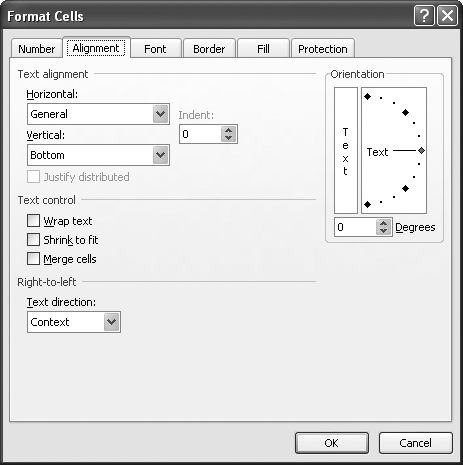
The smallest unit of organization in a worksheet is the cell, which is formed by the intersection of a row and a column. Changing the appearance of individual cells is exactly the same as changing the formatting of a column or row—you select the cells and use the controls on the Home tab of the Ribbon or in the Format Cells dialog box. You can find most of the available cell formatting options on the Home tab, but the Format Cells dialog box offers further possibilities (see Figure 1-11).

Two useful formatting options are controlled by checkboxes in the Text Control section of the Alignment tab: "Wrap text” and "Shrink to fit”. The first forces text in a cell to fit within the left and right borders of a cell. The cell will expand vertically to accommodate its contents. “Shrink to fit” does the opposite, reducing text size until it fits within the cell.

Figure 1-11. The Alignment tab of the Format Cells dialog box lets you control the orientation of text in your cells.

Tip

“Shrink to fit” and “Wrap text” are mutually exclusive; selecting “Wrap text” disables the “Shrink to fit” checkbox, and vice versa.

Finally, just as you can insert and delete columns, you can insert and delete cells. Since inserting or deleting cells can shift the surrounding cells, you can select the direction in which surrounding worksheet cells are pushed. If you add cells, Excel will adjust any existing formulas that reference cells that were moved. If you delete a cell that’s used in a formula, however, the formula will generate an error. You’ll have to edit the formula to reference the appropriate cells.

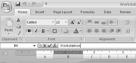
Characters

When you want to change the appearance of a cell’s contents, you just select the cell and have at it. Editing individual characters in a cell isn’t obvious—click the cell and select the characters you want to format in the formula bar at the top of the worksheet (Figure 1-12) or inside the cell itself. The formatting controls on the Home tab of the Ribbon and the Format Cells dialog box are, as always, at your disposal.

Figure 1-12. Edit a cell’s contents either in the cell or the formula bar.

Formatting applied to individual characters overrides formatting applied to the cell as a whole.

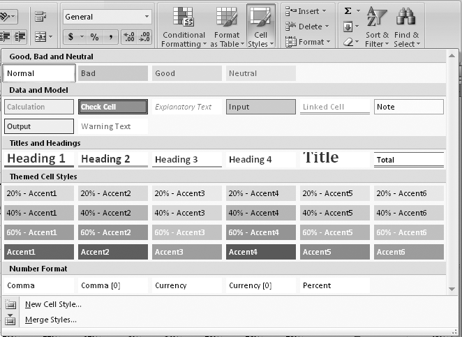
Styles

A style is a prefab format, from alignment to font to borders, that you can apply to a cell. Like Word 2007, Excel 2007 has a substantially larger set of built-in styles than was available in previous versions of Office. To see which styles are available, click Home → Cell Styles, and select from among the different offerings that appear in the Cell Styles gallery (see Figure 1-13).

Figure 1-13. Excel 2007 presents the built-in styles, and any styles you’ve created, in the Cell Styles gallery.

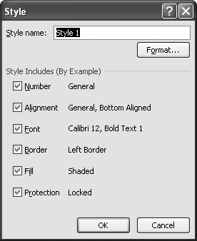
You can, of course, create your own custom cell styles. To do so, click Home → Cell Styles → New Cell Style to display the Style dialog box, shown in Figure 1-14.

When you display the Style dialog box, it shows the details of the style that’s applied to the active cell. When you view a style in here, you see a series of checkboxes indicating how various elements (alignment, font, border, etc.) are formatted in the style. To view the details of a style, click the Format button, which displays all the tabs in the Format Cells dialog box. At this point, you can flip through the tabs and change any element, from font size to disabling protection.

To delete a style, right-click it in the Cell Styles gallery and click Delete. If you’d like to modify an existing style, right-click the style in the Cell Styles gallery and click Modify to display the Style dialog box. As when you create a new style, clicking the Format button in the Style dialog box displays the Format Cells dialog box, which you can use to change the selected format.

Figure 1-14. You can create new Excel 2007 styles by using the controls in the Style dialog box.

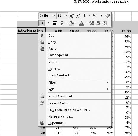
Shortcut Menus and the Mini Toolbar

One handy Windows tool is the right-click menu. Right-clicking an object in a program (such as a cell, row or column header, or sheet tab) displays a short menu of commonly used commands. Microsoft calls these shortcut menus context menus. Figure 1-15 shows the shortcut menu that appears when you right-click a cell.

Here is a quick summary of Excel’s right-click talents:

• Right-clicking a cell displays a shortcut menu with a formatting toolbar you can use to format the cell quickly; editing commands that let you paste, cut, copy, or paste a special item (such as a picture or another workbook) into the cell; commands that let you delete, insert, or clear the contents of the cell; attach a comment; change the cell’s format using the Format Cells dialog box; input a value that already exists in the column; filter or sort worksheet values based on other values in the cell’s column; define the cell as part of a named range; and create a hyperlink.

  

  Figure 1-15. shortcut menu contains buttons and menu items

• Right-clicking a row or column header displays a short-cut menu that contains commands to format the object you right-clicked; cut, copy, paste, and paste special; insert, delete, or clear the contents of the row or column; display the Format Cells dialog box; change the row’s height or the column’s width; as well as options to hide or unhide the row or column.

• Right-clicking a sheet tab lets you insert a new worksheet; delete, rename, hide, move, or copy the sheet you right-clicked; select all sheets; change the worksheet’s tab color; or view the code of any macros attached to the sheet.

• Right-clicking a drawing object lets you format the object quickly using controls on a formatting toolbar; cut, copy, or paste the object; edit the object’s text; change the object’s appearance, size, grouping, and ordering; assign a hyperlink or macro to the object; and assign the shape as the default shape for that workbook.

• Right-clicking a Ribbon button lets you add the button to the Quick Access Toolbar. Similarly, right-clicking a Ribbon group’s name bar (e.g., the Page Setup tab’s Themes group) lets you add the group to the Quick Access Toolbar.

• Right-clicking a button on the Quick Access Toolbar lets you remove the button from the Quick Access Toolbar, customize the Quick Access Toolbar, display the Quick Access Toolbar below the Ribbon (making the Quick Access Toolbar larger), or minimize the Ribbon.

• Right-clicking the status bar (at the very bottom of the window) lets you change the summary operations.

Excel 2007’s shortcut menus have a new item at the top: the Mini Toolbar, which is a small toolbar that contains buttons for the most commonly used formatting commands (e.g., font, font size, font color, fill color, bold, italic, center, etc.). The Mini Toolbar also appears when you select a group of cells and hover your mouse pointer over the selection. Excel 2007 initially draws the Mini Toolbar faintly, but makes it more prominent as you move your mouse pointer closer to it.

How Excel Tries to Help

Excel has a lot going on (you can decide whether that means Excel is “feature rich” or “bloated”), and it should make your life easier. And it does, with several automated features. One useful task Excel performs in the background is saving AutoRecover information—worksheet data, macros, formulas, etc.—so if the program crashes, you lose as little work as possible. There are three other things Excel does in the background (AutoCorrect, AutoComplete, and Smart Tags), but you can turn these—and AutoRecover—off if you wish.

Tip

One thing Excel doesn’t do automatically is highlight suspected spelling and grammar errors in your worksheet. To check spelling, click Review → Spelling.

AutoCorrect

People make the same spelling mistakes again and again, usually those little transpositions (“adn” for “and”) that drive you crazy. Don’t fret. Excel has this and other common misspellings in its list terms to correct automatically.

Tip

If Excel makes a change you don’t want, you can undo the change by pressing Ctrl-Z or clicking the Undo button on the Quick Access Toolbar.

You can add, remove, or redefine AutoCorrect entries by clicking Office Button → Excel Options, clicking the Proofing category head, and then clicking the AutoCorrect Options button. In the dialog box, you can select the types of changes Excel can make or, by unchecking the “Replace text as you type” box, prevent Excel from making any corrections automatically. To add an entry, type the text in the Replace field and the text to replace it in the With field.

ora: If you type in the same lengthy phrases frequently, save your fingers.

You can define an AutoCorrect entry that inserts your boilerplate text whenever you type several letters of the phrase (such as “vty” for “very truly yours”).

Excel also recognizes web addresses and network paths, and automatically formats them as hyperlinks. Excel 2007 also determines whether your entry should be added to an existing Excel table. You can control these options on the “Auto-Format as You Type” tab.

AutoComplete

Most Excel users often enter the same data in a worksheet. For example, if you keep your business’ customer data in a worksheet, many of your customers will probably be from the same state. Excel recognizes repeated values in a column and offers to fill in the expected value. You can turn Auto-Complete on by clicking Office Button → Excel Options, clicking the Advanced category head, and then, in the Editing Options section at the top of the dialog box, checking the “Enable AutoComplete for Cell Values” box.

Smart Tags

Another way Excel automates operations is with Smart Tags. Excel 2007 recognizes specific data in a cell (be it a stock quote or the address of a recently sent email), and tags the cell with a tiny purple notch in the lower-right corner. To turn on Smart Tags, click Office Button → Excel Options, click the Proofing category head, click the Smart Tags tab, and then check the “Label data with smart tags” box.

To test how Smart Tags work, turn them on—enter a stock symbol, for example—hover the pointer over the notch, and then click the Smart Tags action button. You can use the options displayed to summon a fresh quote, a company report on MSN, and more.

Note

You can find more Smart Tags on the Microsoft web site by clicking the More Smart Tags button.