Excel Annoyances

Chapter 4. Manipulating Data Annoyances

Chapters 1 through 3 were all about getting data into Excel, summarizing it, and making it look pretty. In this chapter, you’ll make your data tell you what you need to know—to run a business, to manage a sports team, or to figure out how much money you’ll need to make those mortgage payments.

I’ll start out by showing you how to make your life easy by sorting and filtering your worksheet data. For example, you’ll learn how to create a formula that operates on visible cells only, master multilevel filters, and run sorts that whittle down your data to a manageable size.

Although Excel isn’t a database, you can use it to find values in data lists thanks to the lookup family of formulas. Finally, I’ll dig into PivotTables, the most versatile and useful Excel tool in the book, but one that’s tricky for beginners and annoying for pros. You’ll learn how to avoid the pitfalls when setting up your data, creating PivotTables, analyzing your data, and more.

SORTING AND FILTERING ANNOYANCES

SORT BY VALUES IN MULTIPLE COLUMNS

The Annoyance:

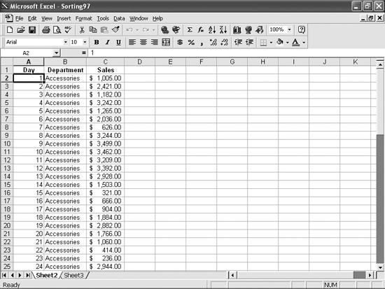
Sorting the data in a single column is so easy, even I figured it out. I just click any cell in the column I want to sort, and then click the Sort Ascending or Sort Descending buttons on the toolbar. But look at my worksheet (Figure 4-1). I recorded my sales data by department (Accessories, Cars, Service), which is a handy enough view. But it doesn’t help me see how I’m doing on a daily basis overall. How can I view my sales data by day?

Figure 4-1. Your sales data is recorded by department—but you need to see sales by day. That means sorting the worksheet by more than one column.

The Fix:

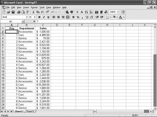
What you need to do is sort the data list by the values in more than one column. Select Data → Sort and use the controls in the Sort dialog box—notably the “Then by” drop downs—to determine the order of the fields and whether to sort each field in ascending or descending order. Sorting by the Day column (in ascending order) and then the Department column (in ascending order) would result in the sorted data list shown in Figure 4-2.

Figure 4-2. In this result, you see all sales, by type, per day.

WHAT’S A DATA LIST?

A data list is a set of data in an Excel worksheet in which each column has a unique name and each row represents a unique datum (for example, a salesperson’s total sales on a given day). There can be no blank rows and no blank columns in the data list, no blank rows between column titles and the data, and no extraneous data in cells neighboring the list. That means you need at least one blank column to the right, at least one blank column (or the edge of the worksheet) to the left, and one blank row at the bottom of the data list. In essence, a data list looks and acts very much like a table in a database. See Figure 4-2 for a typical data list.

SORT DATA BY A CUSTOM SORT ORDER

The Annoyance:

I hate the fact that Excel limits me to sorting data in alphabetical or numerical order! My boss at the car dealership insists the order of importance of our three departments is Cars, Service, and Accessories. He expects the data in my worksheets to reflect that priority, with Cars at the top of the list, Service a close second (if we don’t sell cars, we won’t have anything to fix), and Accessories third. The problem is that Excel insists on sorting the departments only in ascending alpha order (Accessories, Cars, Service), or descending alpha order (Service, Cars, Accessories). I spend a lot of time reordering the data to meet my boss’s requirements. Is there some way I can make Excel sort the department names in an order I define? It would save me hours of work every month.

The Fix:

You’ll probably still have to work the same number of hours per week, but maybe this trick will help you devote those hours to selling cars instead of sorting data. The trick is to create a custom list of values Excel can use as the basis for the sort. The first task is to create a custom list. Here’s how:

1. Type the values you want to sort by in a group of contiguous cells, in a single column or row, in the order you want to sort by. In your case you might type Cars, Service, and Accessories in cells A1, A2, and A3, respectively.

2. Select the cells that contain the values you just typed. Then choose Tools → Options, and click the Custom Lists tab.

3. Verify that the cell range you selected appears in the “Import list from cells” field.

4. Click the Import button and then click OK.

Now you can sort your data in the order of the values in your custom list, but you must use the custom list as the first sorting criterion. To sort your data by the values in your custom list, follow these steps:

1. Click any cell in the data list and press Ctrl-Shift-8 to select the entire list.

2. Choose Data → Sort, and in the Sort dialog box open the “Sort by” drop down and select the column you want to sort using your custom sort order.

3. Click the Options button and in the Sort Options dialog box open the “First key sort order” field, select your custom list from the list, and click OK.

4. If desired, you can set additional sorting criteria. Click OK, and when you return to the Sort dialog box click OK again to sort your data.

SORT DATA LEFT TO RIGHT

The Annoyance:

Excel assumes everyone’s data is arranged in columns, so all the sort functions work that way. However, sometimes I want to sort a row of values. How do I do that?

The Fix:

To sort a row of values, select the row and choose Data → Sort, click the Options button, and in the Orientation section select “Sort left to right,” and click OK. Then open the “Sort by” drop down, select the row you want to sort, select either Ascending or Descending, and click OK.

FILTER WORKSHEET DATA

The Annoyance:

I create huge worksheets. In fact, I have one worksheet that is three columns wide and more than 1,000 rows long. You can see a sample of what I mean in Figure 4-3.

Figure 4-3. This data needs a serious trim.

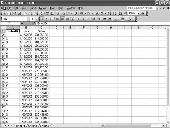
For today, all I want to see are the sales for the rep with SalesID 1. That’s all. Nothing more. Nada mas. Zip. How do I do that?

The Fix:

To display just those rows that contain a certain value, click any cell in the data list. Then select Data → Filter → AutoFilter; a series of down arrows will appear in the first cell of every column in the list. (They hide the values in those cells, too.) These are filter arrows, and clicking one displays a drop-down list of filtering options. Click the value you want to use as your filter. All the rows in which that value does not occur in that column disappear. To refilter the results, click the filter arrow again and select a new criterion from the drop-down list. Incidentally, a filter arrow turns blue when the filter is active.

When you start this process, be sure not to click a column header (Excel’s gray markers that denote column A, B, C, and so on). If you do and then you choose Data → Filter → AutoFilter, Excel will add a filter arrow only to the selected column.

To cancel all the filters, choose Data → Filter → Show All. To get out of filtering mode altogether and remove the filter arrows, choose Data → Filter → AutoFilter again. In Excel 2003, these filtering capabilities are included in the new List feature. For more information on Lists in Excel 2003, see the section "Excel 2003 List Annoyances" in Chapter 9.

DISPLAY TOP OR BOTTOM VALUES

The Annoyance:

I use a long, complicated worksheet that shows hourly sales results for the auto dealership where I work. Instead of spending hours with a calculator to find the top 10 car-sales hours in the list, I was hoping there was some way I could get Excel to do that for me. Is there?

The Fix:

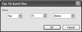
When you click the filter arrow in the top row of your data list (see previous item), you’ll see a set of filtering options. One of those options is Top 10, which displays the Top 10 AutoFilter dialog box (shown in Figure 4-4). You can use the controls to determine whether you want to display the top or bottom values from the list, and the number of values to display. You also can choose whether the number in the middle box represents a number of list entries to display, or the percentage of entries to display. For example, if you type 10 in the middle box, and in the far right box you select Percent, Excel will display the top 10% of the values in that column.

Figure 4-4. Find the best and worst in a list using a Top 10 AutoFilter.

CREATE A MULTILEVEL FILTER

The Annoyance:

The other day, when I was giving a presentation based on the same auto dealership worksheet, one of the owners wanted to see a list of just those hours during which accessory sales were more than $2,500. I ended up sorting the list by department and then by sales in descending order, but it took forever and my boss was drumming his fingers by the end. Isn’t there a faster way to filter list data by a criterion?

The Fix:

To filter your data by a criterion, choose Data → Filter → AutoFilter, click the filter arrow at the top of the column to which you want to assign the criterion, and choose Custom to display the Custom AutoFilter dialog box (shown in Figure 4-5).

Figure 4-5. Filter your data by values in more than one column? Sure!

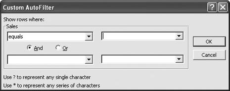
You can use the controls in the Custom AutoFilter dialog box to create two criteria by which you want to filter your data. When you open the top-left drop down, you’ll see a list of Boolean operators (less than, greater than or equal to, and so on) to use on your data, while the top-right drop down contains a list of values taken from the column. (You can type in your own value if you want.) For example, if you wanted to find all hours during which sales were more than $2,500, you could choose “is greater than” in the top-left drop down and type 2500 in the top-right drop down.

If you want to create more complex criteria, dig into the second set of fields in the Custom AutoFilter dialog box and select the And or the Or radio buttons. For example, to find all sales hours with totals of more than $2,500 or less than $500, you would select the Or option, then choose “is less than” in the bottom-left drop down and type 500 in the bottom-right drop down.

The Custom AutoFilter you create filters values from only one column at a time, but you can use another filter to further hone the results the AutoFilter displays. To limit the results to the Accessories department, for example, you would click the Department filter arrow, choose Accessories from the value list, and then apply the custom filter.

FIND DUPLICATE ENTRIES IN A DATA LIST

The Annoyance:

I am frustrated! I have a spreadsheet with 8,500 addresses that I’m going to use for an upcoming postcard mailing, but I need to pare the list to about 5,000 or I’ll blow my postage budget. A lot of those 8,500 entries are duplicates, but Excel stubbornly refuses to find them for me. A friend told me I could export the data list to Access and run a Find Duplicates query. Please don’t tell me I have to learn Access!

The Fix:

Although finding duplicate entries per se requires a VBA macro, you can use the Advanced Filter dialog box (shown in Figure 4-6) to copy the unique rows from a data list to another location in your workbook—handily leaving all the duplicate entries behind.

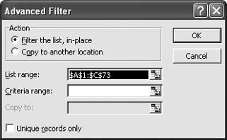
Figure 4-6. The Advanced Filter dialog box: not nearly as advanced as you might think, and quite useful.

To copy just the unique records in a data list, follow these steps:

1. Choose Data → Filter → Advanced Filter.

2. Select Copy to Another Location.

3. Click the Collapse Dialog button in the “List range” field and highlight the cells you want to filter, then press Enter.

4. Click the Collapse Dialog button in the “Copy to” field and click the cell at the top left of the range where you want to paste the filtered list (I suggest cell A1 of a blank worksheet). Press Enter.

5. Check the “Unique records only” checkbox and click OK.

Excel must find an exact match, including all punctuation, for two entries to be considered the same. If this doesn’t whittle down your list much and you suspect there might be some undetected duplicate entries, try sorting the address list by last name, first name, and postal code to help simplify your job of spotting duplicates.

COPY ONLY VISIBLE CELLS FROM A FILTERED LIST

The Annoyance:

I filtered a data list (shown in Figure 4-7), but when I try to copy the filtered rows and paste them into another worksheet, Excel pastes the hidden rows as well. I can tell I’ve selected more than the visible cells because as I select the cells, the Name box tells me I’ve selected an area that’s 74 rows by 5 columns. How do I copy and paste just the visible rows in my data list?

Figure 4-7. If you want to copy just the visible cells, use the Select Visible Cells button.

The Fix:

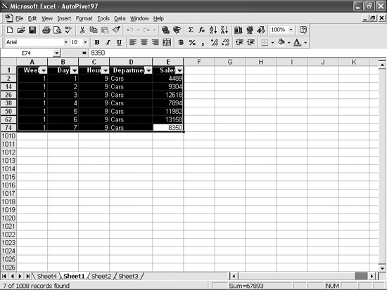
To copy just the visible cells to the clipboard, you need to add the Select Visible Cells button to your toolbar. To add this button, choose Tools → Customize, select the Commands tab, select Edit from the Categories list, scroll down in the righthand Commands list until you find the Select Visible Cells button, and drag the button to any toolbar. Then, to copy and paste just the visible cells, follow these steps:

1. Filter the data list and highlight the visible cells.

2. Click the Select Visible Cells toolbar button.

3. Select Edit → Copy.

4. Choose Edit → Paste.

RUBIK’S CUBE IN EXCEL

If you ever played with a Rubik’s Cube, raise your hand. Wow, a lot of hands are in the air!

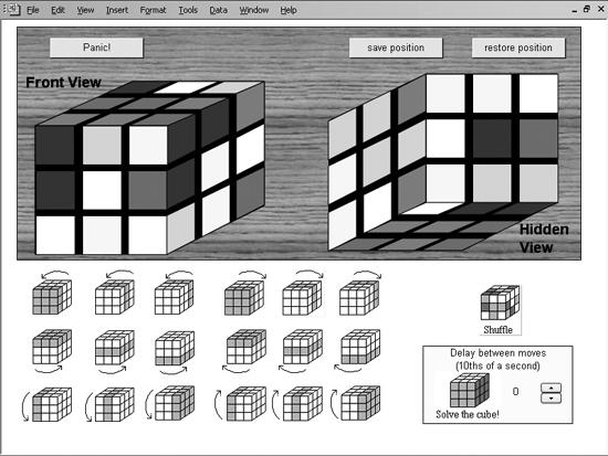
If you feel funny about having toys lying around your office, but would enjoy an occasional diversion that tests your visualization and problem-solving skills, download the free Rubik’s Cube emulator (written by Robin Glynn) from http://www.xl-logic.com/xl_files/games/cube.zip. All you need to do is unzip the zip file and open the cube.xls workbook. As you can see in the figure, you manipulate the cube by clicking the renderings of the cube at the bottom of the screen representing the move you want to make. Buttons on the right side of the workbook save your position, restore a saved position, shuffle the cube’s position randomly, and solve the cube automatically. You also can control how quickly the computer manipulates the cube in auto-solve mode. Don’t change the time between moves while the algorithm is running, though. I managed to freeze my computer for two minutes when I tried.

In the great tradition of workplace entertainment, there’s a Panic button that closes the workbook immediately. You’ll lose your position in the game, but you’ll keep your position at work.

Figure 4-8. Twist your mind by twisting a cube.

SUMMARIZE VISIBLE CELLS ONLY

The Annoyance:

Filters work for me, but I can’t figure out how to create a formula that only summarizes the visible data in a worksheet. For example, let’s say I’m working with sales data. I need to total the sales for each representative, but I can’t find a way to add the cells for each representative without creating formulas that pinpoint individual cells. For instance, when I worked with the worksheet shown in Figure 4-3, I needed to create a formula that added cells C2, C5, C9, C12, C17, and C22 to find out the total for the salesperson with the SalesID 1. Then I had to add the values in cells C3, C10, C13, C18, and C23 for salesperson 2, and so on. I can filter the data list to show just one sales rep’s sales. Can’t I create a formula that totals just those cells?

The Fix:

Figuring out what to do when your data doesn’t behave is one of the most annoying aspects of working with Excel. Fortunately, in this case, the fix is actually fairly straightforward. You can create a filter that enables you to pick the sales representative whose data you want to summarize, and then create a Subtotal formula in a cell below the sales data. Here’s the procedure in more detail:

1. Click any cell in the data list (in Figure 4-3, the data list is the cell range A1:C26).

2. Choose Data → Filter → AutoFilter.

3. Click the SalesID down arrow and click a SalesID number.

4. Click a cell in the Sales column that is below the data.

5. Click the AutoSum button on Excel’s standard toolbar and press Enter.

Usually when you click the AutoSum toolbar button, you create a vanilla Sum formula that adds the data in every cell in your selected range and places the result just below. But if you click the AutoSum toolbar button in a cell below a filtered column of data, Excel creates a Subtotal formula. What’s the difference? If you create a Subtotal formula below a filtered list when the filter is in place, the formula only calculates its total (or average, or minimum, or maximum, or whatever) based on the cells that are visible in a filtered list.

The Subtotal formula has the syntax =SUBTOTAL( function, range ), where function is the number of the summary calculation to be performed on the data and range is the range of cells in the filtered column. Table 4-1 lists the summary operations available to you when you create a SUBTOTAL() formula.

Table 4-1. Summarizing data with a SUBTOTAL ( ) formula.

Number	Function
1	AVERAGE (the numeric average of the visible cells)
2	COUNT (the number of visible cells)
3	COUNTA (the number of visible cells that contain a value)
4	MAX (the maximum value in the visible cells)
5	MIN (the minimum value in the visible cells)
6	PRODUCT (the multiplicative product of the values in the visible cells)
7	STDEV (the standard deviation of the values in the visible cells)
8	STDEVP (the standard deviation of every cell named in the formula)
9	SUM (the arithmetic sum of the values in the visible cells)
10	VAR (the variance of the values in the visible cells)
11	VARP (the variance of every cell named in the formula)