Excel Annoyances

WHAT-IF ANALYSIS ANNOYANCES

CREATE A SCENARIO

The Annoyance:

I have two bosses, which means I’m asked a lot of “What if” questions. For example, when I put together a project cost summary worksheet, each boss asked about different sets of variables: what would be the effect if one component or another cost more or less? Could I drive down labor costs through productivity gains? All good questions, but when I try to include them in one worksheet my head starts spinning. What I really need is some way to display alternative values in certain selected cells, such as labor costs and component prices, and a way to switch back and forth between them. Is that possible?

The Fix:

You have only two bosses? Luxury. When I worked in Washington, DC, I had two official bosses and three “dotted-line” bosses who could reach across the corporate organization chart to order me around. Needless to say, I developed a few survival strategies, and one of them is the scenario.

A scenario is an alternative data set you can store as part of a worksheet. When you want to display the alternative values, just call up the alternate scenario and keep right on going with your presentation. Here’s how you create a scenario:

1. Choose Tools → Scenarios to display the Scenario Manager dialog box.

2. Click the Add button, and give your new scenario a name.

3. Click the Collapse Dialog button in the “Changing cells” field, select the cells you want to change, and press Enter. Remember that you can select noncontiguous groups of cells by holding down the Ctrl key when you select the cells. Click OK when you’re done.

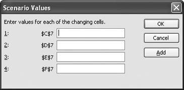
4. In the Scenario Values dialog box (shown in Figure 4-16) enter the new values for your selected cells. Click OK to close the dialog box and then click the Close button to close the Scenario Manager dialog box.

Figure 4-17. Enter your new scenario values here...

To apply a scenario, follow these steps:

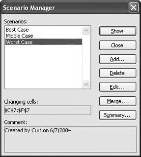
1. Choose Tools → Scenarios to display the Scenario Manager dialog box (shown in Figure 4-17).

   

   Figure 4-18. ...and display them here.

2. Click the name of the scenario to display, and click the Show button.

3. Click Close to close the Scenario Manager dialog box.

When you want to hide the scenario, just click the Undo button on Excel’s standard toolbar.

Warning: never use scenarios in any workbook that holds the only copy of your data. Instead, make a backup copy of the workbook to use for your scenario what-if analyses. Here’s why: unless you carefully undo the scenario change, Excel leaves the values from the last-active scenario in place. If you close your worksheet without restoring the original values by clicking the Undo button, Excel will overwrite the original values! As a second safety measure, create a Normal scenario that contains the original values of every cell affected by one of your scenarios. Scenarios are limited to 32 cell changes each, so you might need to create more than one scenario to hold your original values, but the work is worth it to make sure your original data remains intact.

FIND A VALUE THAT GENERATES A SPECIFIC RESULT

The Annoyance:

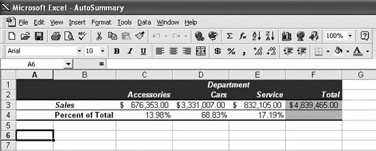
I created a summary table that lists the total revenue from the Accessories, Car, and Service departments at my auto dealership (see Figure 4-18). I’m disappointed that the Service department isn’t pulling its weight; in most dealerships the Service department makes up at least 20% of the total revenue. So, how much more do I have to make from Service to get its total up to 20%? I probably could create some complicated formula, or fake it by plugging in dozens of different service revenue numbers until I finally got the share to exactly 20%, but is there some way Excel can do it for me?

Figure 4-19. Don’t chase your data’s tail! Let Excel do the work for you.

The Fix:

To find a value that will generate a specific formula result, follow these steps:

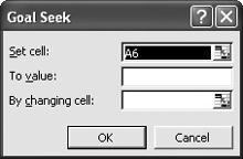
1. Choose Tools → Goal Seek to display the Goal Seek dialog box (shown in Figure 4-19).

   

   Figure 4-20. Set your goals, and Excel will see if it’s possible to meet them.

2. With your cursor in the “Set cell” field, click the Collapse Dialog button on the right side of the field and click the cell with the formula that you want to generate a specific result (in the example, that’s cell E4).

3. In the “To value” field, type the value you want the formula to generate (in this example, that would be either .2 or 20%).

   BEWARE OF PERCENTAGES IN GOAL SEEK

   When you’re working with percentages in Goal Seek, it’s easy to type in the wrong value. In this case, you might mistakenly type 20 in the “To value” field instead of .2 or 20%. If you make this mistake, Goal Seek will attempt to find a value for cell E3 that made it 20 times larger than (or 2000% of) the value in F3. This is impossible, of course, because cell E4 generates its value by dividing one department’s sales by the total of all departments’ sales, which means the value in cell F3, the grand total, always will be larger than the value in cell E3, one department’s total.

4. With your cursor in the “By changing cell” field, click the Collapse Dialog button on the right side of the field and click the cell in the worksheet that holds the formula input you want to change (in this example, that would be cell E3). Then click the Expand Dialog button, and click OK.

5. Excel displays the solution, if any, to the problem. You can either click OK to replace the existing worksheet values with the result, or click Cancel to return to the original values.

To find out how to use Goal Seek with Excel charts, see the annoyance "Seeking Your Goal with a Chart" in Chapter 5.

USE SOLVER TO SOLVE MULTIVARIATE PROBLEMS

The Annoyance:

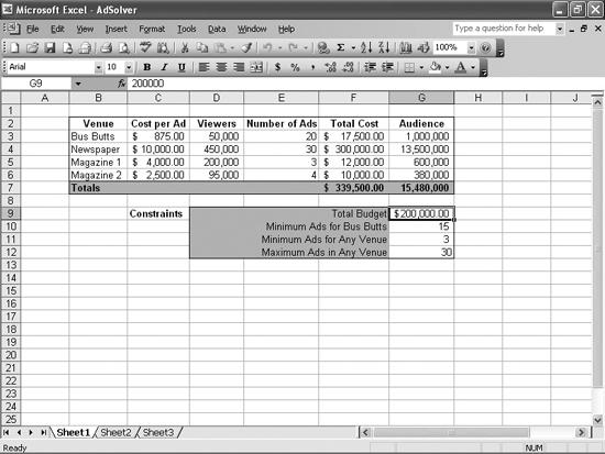
I believe my annoyances extend far beyond the abilities of Goal Seek, but hey, maybe I’m wrong. Basically, I’m trying to figure out the best mix of advertisements for my company:

• I want to put my ads in front of as many people as possible.

• I have an advertising budget of $200,000.

• I must buy at least 15 ads on the backs of buses (“bus butts”) to fulfill my end of a deal with the city.

• I must buy at least three ads in the lowest-circulation magazine to keep the editor (my brother-in-law) happy.

• I don’t want to buy more than 30 ads in any venue.

• I can’t buy a fraction of an ad, so the varying cells must contain integer values.

So, given the venue, price, and viewership figures in Figure 4-20, how do I figure out the best advertising mix for my business?

The Fix:

Goal Seek works only when you want to vary the value in a single cell. To solve problems wher you might need to vary the value in multiple cells, you need to move up to Solver, which is an Excel add-in produced by Frontline Systems and included for free with Excel. To check if Solver is installed, click Tools and see if there’s a Solver item about halfway down the menu. If there isn’t, choose Tools → Add-Ins, check the Solver Add-In box, and click OK to install Solver. If Solver is not listed in the Add-Ins dialog box, open the Windows Start menu, choose Search → For Files or Folders (or Find, depending on your OS), and search for the file Solver.xla. If you find it, in Excel choose Tools → Add-Ins, click the Browse button, and navigate to the file. If you can’t locate the file, you might need to run the Office setup program to add the Solver component.

Figure 4-21. Make your assumptions clear so that Excel can understand them.

Once Solver is installed, choose Tools → Solver to display the Solver Parameters dialog box (shown in Figure 4-21).

Figure 4-22. The base station for Solver in its natural state.

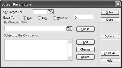
You’ll use the Solver Parameters dialog box to enter the rules for your problem. Put your assumptions in the worksheet along with your data—they’ll be easier to find in the Solver Parameters dialog box.

Here are the steps to create the model described in the annoyance:

1. Select cell G7, which is the cell with the value you want to maximize (total audience), and choose Tools → Solver. The Solver Parameters dialog box will appear with cell G7 already indicated in the Target Cell field.

2. In the By Changing Cells field, click the Collapse Dialog button, select cells E3:E6, and click the Expand Dialog button.

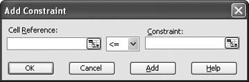
3. Click the Add button to display the Add Constraint dialog box (shown in Figure 4-22).

   

   Figure 4-23. Don’t let your data get out of line... constrain it!

4. To add the rule that the number of ads bought must be an integer value, click the Collapse Dialog button, select cells E3:E6, and click the Expand Dialog button. Then open the middle drop down in the dialog, select “int,” and click the Add button. Note: if you plan to use this constraint, always add the rule first. When I first entered this solution, I created the “every ad buy must be an integer” rule last and, for some reason, got the value 29.065 for the Magazine 1 ad buy. When I deleted the scenario and reentered it, creating the “must be an integer” rule first, the solution came out all integers, the way I wanted it to. The lesson? Excel processes constraints in the order you enter them, so you always should put your formatting constraints (e.g., this value must be an integer) before the value-related constraints.

5. With your cursor in the Cell Reference field, click the Collapse Dialog button, select cell F7, and click the Expand Dialog button. Then select “<=” in the middle drop down, in the Constraint field select cell G9, and then click the Add button.

6. With your cursor in the Cell Reference field, click the Collapse Dialog button, select cells E3:E6, and click the Expand Dialog button. Then open the middle drop down, select “>=”, in the Constraint field select cell G11, and then click the Add button.

7. With your cursor in the Cell Reference field, click the Collapse Dialog button, select cell E3, and click the Expand Dialog button. Then open the middle drop down, select “>=”, in the Constraint field select cell G10, and then click the Add button.

8. With your cursor in the Cell Reference field, click the Collapse Dialog button, select cells E3:E6, and click the Expand Dialog button. Then open the middle drop down and select “<=”. In the Constraint field, select cell G12, and click OK to display the Solver Parameters dialog box with your constraints.

9. Click Solve.

If you make a mistake while creating any of the criteria, you can click the rule in the “Subject to the Constraints” section of the Solver Parameters dialog box and click the Change button to edit the rule.

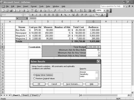
If Solver can find a solution to your problem, it will change the values in your worksheet and display a success message in the Solver Results dialog box, shown in Figure 4-23.

You can elect to keep the Solver values, or restore the original values, by selecting the appropriate option. If you want to save the Solver values as a scenario, click the Save Scenario button and type in a name for the new scenario.

Figure 4-24. Another happy ending—Solver returns just the results you needed.

PLACE DATA ANALYSIS ON A MENU

The Annoyance:

I’m trying to do some advanced data analysis (regression and such), and the boss left me instructions to “open the Tools menu and click Data Analysis.” But there is no Data Analysis item on my Tools menu. And please don’t tell me I have to buy something extra!

The Fix:

You don’t have to buy anything extra, but you do need to install the Data Analysis add-in that comes standard with the program. To do so, choose Tools → Add-Ins, check the Analysis ToolPak and (for good measure) the Analysis ToolPak-VBA boxes, and click OK. Excel will add the Data Analysis item to the Tools menu, so you can use the additional statistical functions to analyze your data.