Financial Markets and Trading: An Introduction to Market Microstructure and Trading Strategies

APPENDIX B

Elements of Time Series Analysis

The methods of time series analysis are the main tools used for analysis of price dynamics, as well as for formulating and back-testing trading strategies. Here, we present an overview of the concepts used in this book. For more details, readers can consult Alexander (2001), Hamilton (1994), Taylor (2005), and Tsay (2005).

THE AUTOREGRESSIVE MODEL

First, we consider a univariate time series y(t) that is observed at moments t = 0, 1, …, n. The time series in which the observation at moment t takes place depends linearly on several lagged observations at moments t − 1, t − 2, …, t − p

is called the autoregressive process of order p, or AR(p). The white noise ε(t) satisfies the following conditions:

The lag operator L^p = y(t − p) is often used in describing time series. Note that L⁰ = y(t). Equation (B.1) in terms of the lag operator,

has the form

It is easy to show for AR(1) that

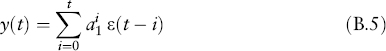
Obviously, contributions of old noise converge with time to zero ...