iPhone 3D Programming

Chapter 2. Math and Metaphors

There’s a pizza place near where I live that sells only slices. In the back you can see a guy tossing a triangle in the air.

—Stephen Wright, comedian

Computer graphics requires more mathematics than many other fields in computer science. But if you’re a pragmatic OpenGL programmer, all you really need is a basic grasp of linear algebra and an understanding of a few metaphors.

In this chapter, I explain these metaphors and review the relevant linear algebra concepts. Along the way I’ll tick off various OpenGL functions that relate to these concepts. Several of such functions were used in the HelloArrow sample, so code that may have seemed mysterious should now become clear.

Near the end of the chapter, we’ll leverage these math concepts to push the HelloArrow sample into the third dimension, transforming it into HelloCone.

The Assembly Line Metaphor

You can think of any graphics API, including OpenGL ES, as an assembly line that takes an assortment of raw materials such as textures and vertices for input and eventually produces a neatly packaged grid of colors.

The inputs to the assembly line are the natural starting points for learning OpenGL, and in this chapter we’ll focus on vertices. Figure 2-1 depicts the gradual metamorphosis of vertices into pixels. First, a series of transformations is performed on the vertices; next the vertices are assembled into primitives; and finally, primitives are rasterized into pixels.

Figure 2-1. The OpenGL ES assembly line

Note

At a high level, Figure 2-1 applies to both OpenGL ES 1.1 and 2.0, but it’s important to note that in 2.0, the Transforms block contains a vertex shader, and the Rasterization block hands his output over to a fragment shader.

In this chapter we’ll mostly focus on the transformations that occur early on in the assembly line, but first we’ll give a brief overview of the primitive assembly step, since it’s fairly easy to digest.

Assembling Primitives from Vertices

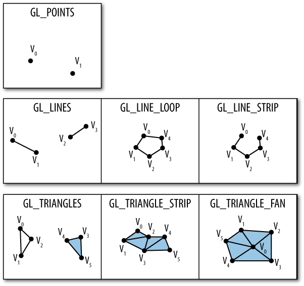
The 3D shape of an object is known as its geometry. In OpenGL, the geometry of an object constitutes a set of primitives that are either triangles, points, or lines. These primitives are defined using an array of vertices, and the vertices are connected according to the primitive’s topology. OpenGL ES supports seven topologies, as depicted in Figure 2-2.

Figure 2-2. Primitive topologies

Recall the one line of code in HelloArrow from Chapter 1 that tells OpenGL to render the triangles to the backbuffer:

glDrawArrays(GL_TRIANGLES, 0, vertexCount);

The first argument to this function specifies the primitive topology: GL_TRIANGLES tells OpenGL to interpret the vertex buffer such that the first three vertices compose the first triangle, the second three vertices compose the second triangle, and so on.

In many situations you need to specify a sequence of adjoining triangles, in which case several vertices would be duplicated in the vertex array. That’s when GL_TRIANGLE_STRIP comes in. It allows a much smaller set of vertices to expand to the same number of triangles, as shown in Table 2-1. In the table, v is the number of vertices, and p is the number of primitives. For example, to draw three triangles using GL_TRIANGLES, you’d need nine vertices (3p). To draw them using GL_TRIANGLE_STRIP, you’d need only five (p + 2).

Table 2-1. Primitive counts

Topology	Number of primitives	Number of vertices
GL_POINTS	v	p
GL_LINES	v / 2	2p
GL_LINE_LOOP	v	p
GL_LINE_STRIP	v - 1	p + 1
GL_TRIANGLES	v / 3	3p
GL_TRIANGLE_STRIP	n - 2	p + 2
GL_TRIANGLE_FAN	n - 1	p + 1

Another way of specifying triangles is GL_TRIANGLE_FAN, which is useful for drawing a polygon, a circle, or the top of a 3D dome. The first vertex specifies the apex while the remaining vertices form the rim. For many of these shapes, it’s possible to use GL_TRIANGLE_STRIP, but doing so would result in degenerate triangles (triangles with zero area).

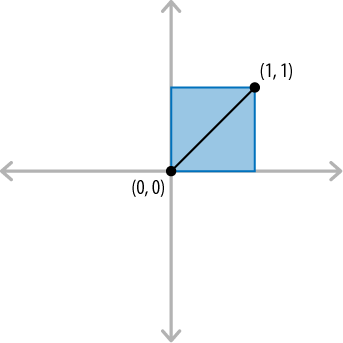
For example, suppose you wanted to draw a square shape using two triangles, as shown in Figure 2-3. (Incidentally, full-blown OpenGL has a GL_QUADS primitive that would come in handy for this, but quads are not supported in OpenGL ES.) The following code snippet draws the same square three times, using a different primitive topology each time:

const int stride = 2 * sizeof(float);

float triangles[][2] = { {0, 0}, {0, 1}, {1, 1}, {1, 1}, {1, 0}, {0, 0} };
glVertexPointer(2, GL_FLOAT, stride, triangles);
glDrawArrays(GL_TRIANGLES, 0, sizeof(triangles) / stride);

float triangleStrip[][2] = { {0, 1}, {0, 0}, {1, 1}, {1, 0} };
glVertexPointer(2, GL_FLOAT, stride, triangleStrip);
glDrawArrays(GL_TRIANGLE_STRIP, 0, sizeof(triangleStrip) / stride);

float triangleFan[][2] = { {0, 0}, {0, 1}, {1, 1}, {1, 0} };
glVertexPointer(2, GL_FLOAT, stride, triangleFan);
glDrawArrays(GL_TRIANGLE_FAN, 0, sizeof(triangleFan) / stride);

Figure 2-3. Square from two triangles

Triangles aren’t the only primitive type supported in OpenGL ES. Individual points can be rendered using GL_POINTS. The size of each point can be specified individually, and large points are rendered as squares. Optionally, a small bitmap can be applied to each point; these are called point sprites, and we’ll learn more about them in Chapter 7.

OpenGL supports line primitives using three different topologies: separate lines, strips, and loops. With strips and loops, the endpoint of each line serves as the starting point for the following line. With loops, the starting point of the first line also serves as the endpoint of the last line. Suppose you wanted to draw the border of the square shown in Figure 2-3; here’s how you could do so using the three different line topologies:

const int stride = 2 * sizeof(float);
	
float lines[][2] = { {0, 0}, {0, 1},
                     {0, 1}, {1, 1},
                     {1, 1}, {1, 0},
                     {1, 0}, {0, 0} };
glVertexPointer(2, GL_FLOAT, stride, lines);
glDrawArrays(GL_LINES, 0, sizeof(lines) / stride);

float lineStrip[][2] = { {0, 0}, {0, 1}, {1, 1}, {1, 0}, {0, 0} };
glVertexPointer(2, GL_FLOAT, stride, lineStrip);
glDrawArrays(GL_LINE_STRIP, 0, sizeof(lineStrip) / stride);

float lineLoop[][2] = { {0, 0}, {0, 1}, {1, 1}, {1, 0} };
glVertexPointer(2, GL_FLOAT, stride, lineLoop);
glDrawArrays(GL_LINE_LOOP, 0, sizeof(lineLoop) / stride);

Associating Properties with Vertices

Let’s go back to the assembly line and take a closer look at the inputs. Every vertex that you hand over to OpenGL has one or more attributes, the most crucial being its position. Vertex attributes in OpenGL ES 1.1 can have any of the forms listed in Table 2-2.

Table 2-2. Vertex attributes in OpenGL ES

Attribute	OpenGL enumerant	OpenGL function call	Dimensionality	Types
Position	GL_VERTEX_ARRAY	glVertexPointer	2, 3, 4	byte, short, fixed, float
Normal	GL_NORMAL_ARRAY	glNormalPointer	3	byte, short, fixed, float
Color	GL_COLOR_ARRAY	glColorPointer	4	ubyte, fixed, float
Point Size	GL_POINT_SIZE_ARRAY_OES	glPointSizePointerOES	1	fixed, float
Texture Coordinate	GL_TEXTURE_COORD_ARRAY	glTexCoordPointer	2, 3, 4	byte, short, fixed, float
Generic Attribute (ES 2.0)	N/A	glVertexAttribPointer	1, 2, 3, 4	byte, ubyte, short, ushort, fixed, float

With OpenGL ES 2.0, only the last row in Table 2-2 applies; it needs you to define your own custom attributes however you see fit. For example, recall that both rendering engines in HelloArrow enabled two attributes:

// OpenGL ES 1.1
glEnableClientState(GL_VERTEX_ARRAY);
glEnableClientState(GL_COLOR_ARRAY);

// OpenGL ES 2.0
glEnableVertexAttribArray(positionSlot);
glEnableVertexAttribArray(colorSlot);

The ES 1.1 backend enabled attributes using constants provided by OpenGL, while the ES 2.0 backend used constants that were extracted from the shader program (positionSlot and colorSlot). Both backends specified the dimensionality and types of the vertex attributes that they enabled:

// OpenGL ES 1.1 
glVertexPointer(2, GL_FLOAT, ... );
glColorPointer(4, GL_FLOAT, ... );

// OpenGL ES 2.0
glVertexAttribPointer(positionSlot, 2, GL_FLOAT, ...);
glVertexAttribPointer(colorSlot, 4, GL_FLOAT, ...);

The data type of each vertex attribute can be one of the forms in Table 2-3. With ES 2.0, all of these types may be used; with ES 1.1, only a subset is permitted, depending on which attribute you are specifying (see the far right column in Table 2-2).

Table 2-3. Vertex attribute data types

OpenGL type	OpenGL enumerant	Typedef of	Length in bits
GLbyte	GL_BYTE	signed char	8
GLubyte	GL_UNSIGNED_BYTE	unsigned char	8
GLshort	GL_SHORT	short	16
GLushort	GL_UNSIGNED_SHORT	unsigned short	16
GLfixed	GL_FIXED	int	32
GLfloat	GL_FLOAT	float	32

The position attribute in OpenGL ES 1.1 is a bit of a special case because it’s the only required attribute. It can be specified as a 2D, 3D, or 4D coordinate. Internally, the OpenGL implementation always converts it into a 4D floating-point number.

Four dimensional? This might conjure images of Dr. Who, but it actually has nothing to do with time or anything else in physics; it’s an artificial construction that allows all transformations to be represented with matrix multiplication. These 4D coordinates are known as homogeneous coordinates. When converting a 3D coordinate into a homogeneous coordinate, the fourth component (also known as w) usually defaults to one. A w of zero is rarely found but can be taken to mean “point at infinity.” (One of the few places in OpenGL that uses w = 0 is light source positioning, as we’ll see in Chapter 4.) Specifying a vertex with a negative w is almost never useful.

Homogeneous Coordinates

Homogeneous coordinates came into existence in 1827 when August Ferdinand Möbius published Der barycentrische Calcül. This is the same Möbius of Möbius strip fame. Just for fun, we’ll discuss how to render a Möbius strip later in this book. Incidentally, Möbius also invented the concept of barycentric coordinates, which is leveraged by the graphics chip in your iPhone when computing the interior colors of triangles. This term stems from the word barycentre, the archaic word for center of mass. If you place three weights at the corners of a triangle, you can compute the balance point using barycentric coordinates. Their derivation is beyond the scope of this book but an interesting aside nonetheless!

So, shortly after entering the assembly line, all vertex positions become 4D; don’t they need to become 2D at some point? The answer is yes, at least until Apple releases an iPhone with a holographic screen. We’ll learn more about the life of a vertex and how it gets reduced to two dimensions in the next section, but for now let me mention that one of the last transformations is the removal of w, which is achieved as shown in Equation 2-1.

Equation 2-1. Perspective transform

This divide-by-w computation is known as the perspective transform. Note that we didn’t discard z; it’ll come in handy later, as you’ll see in Chapter 4.

The Life of a Vertex

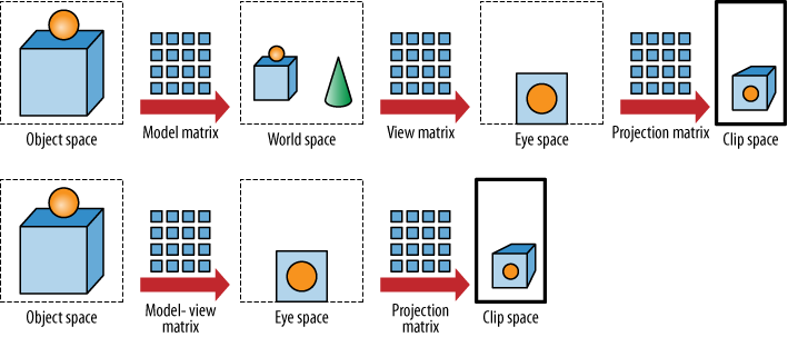
Figure 2-4 and Figure 2-5 depict the process of how a vertex goes from being 4D to being 2D. This portion of the assembly line is commonly known as transform and lighting, or T&L. We’ll discuss lighting in Chapter 4; for now let’s focus on the transforms.

After each transform, the vertex is said to be in a new “space.” The original input vertices are in object space and are called object coordinates. In object space, the origin typically lies at the center of the object. This is also sometimes known as model space.

When object coordinates are transformed by the model-view matrix, they enter eye space. In eye space, the origin is the camera position.

Next, the vertex position is transformed by the projection matrix to enter clip space. It’s called clip space because it’s where OpenGL typically discards vertices that lie outside the viewing frustum. This is one of the places where the elusive W component comes into play; if the X or Y components are greater than +W or less than -W, then the vertex is clipped.

Figure 2-4. Early life of a vertex. Top row is conceptual; bottom row is OpenGL’s view

With ES 1.1, the steps in Figure 2-4 are fixed; every vertex must go through this process. With ES 2.0, it’s up to you to do whatever transforms you’d like before clip space. Typically you’ll actually want to perform these same transforms anyway.

After clipping comes the perspective transform mentioned earlier in the chapter. This normalizes the coordinates to [-1, +1], so they’re known as normalized device coordinates at this point. Figure 2-5 depicts the transforms that take place after clip space. Unlike the steps in Figure 2-4, these transforms are integral to both ES 1.1 and ES 2.0.

Figure 2-5. Last three stages of a vertex before rasterization

The last transform before rasterization is the viewport transform, which depends on some values supplied from the application. You might recognize this line from GLView.mm in HelloArrow:

glViewport(0, 0, CGRectGetWidth(frame), CGRectGetHeight(frame));

The arguments to glViewport are left, bottom, width, and height. On the iPhone you’ll probably want width and height to be 320 and 480, but to ensure compatibility with future Apple devices (and other platforms), try to avoid hardcoding these values by obtaining the width and height at runtime, just like we did in HelloArrow.

The glViewport function controls how X and Y transform to window space (somewhat inaptly named for mobile devices; you’ll rarely have a nonfullscreen window!). The transform that takes Z into window space is controlled with a different function:

glDepthRangef(near, far);

In practice, this function is rarely used; its defaults are quite reasonable: near and far default to zero and one, respectively.

So, you now have a basic idea of what happens to vertex position, but we haven’t yet discussed color. When lighting is disabled (as it is by default), colors are passed straight through untouched. When lighting is enabled, these transforms become germane again. We’ll discuss lighting in detail in Chapter 4.

The Photography Metaphor

The assembly line metaphor illustrates how OpenGL works behind the scenes, but a photography metaphor is more useful when thinking about a 3D application’s workflow. When my wife makes an especially elaborate Indian dinner, she often asks me to take a photo of the feast for her personal blog. I usually perform the following actions to achieve this:

1. Arrange the various dishes on the table.

2. Arrange one or more light sources.

3. Position the camera.

4. Aim the camera toward the food.

5. Adjust the zoom lens.

6. Snap the picture.

It turns out that each of these actions have analogues in OpenGL, although they typically occur in a different order. Setting aside the issue of lighting (which we’ll address in a future chapter), an OpenGL program performs the following actions:

1. Adjust the camera’s field-of-view angle; this is the projection matrix.

2. Position the camera and aim it in the appropriate direction; this is the view matrix.

3. For each object:

   1. Scale, rotate, and translate the object; this is the model matrix.

   2. Render the object.

The product of the model and view matrices is known as the model-view matrix. When rendering an object, OpenGL ES 1.1 transforms every vertex first by the model-view matrix and then by the projection matrix. With OpenGL ES 2.0, you can perform any transforms you want, but it’s often useful to follow the same model-view/projection convention, at least in simple scenarios.

Later we’ll go over each of the three transforms (projection, view, model) in detail, but first we need to get some preliminaries out of the way. OpenGL has a unified way of dealing with all transforms, regardless of how they’re used. With ES 1.1, the current transformation state can be configured by loading matrices explicitly, like this:

float projection[16] = { ... };
float modelview[16] = { ... };

glMatrixMode(GL_PROJECTION);
glLoadMatrixf(projection);

glMatrixMode(GL_MODELVIEW);
glLoadMatrixf(modelview);

With ES 2.0, there is no inherent concept of model-view and projection; in fact, glMatrixMode and glLoadMatrixf do not exist in 2.0. Rather, matrices are loaded into uniform variables that are then consumed by shaders. Uniforms are a type of shader connection that we’ll learn about later, but you can think of them as constants that shaders can’t modify. They’re loaded like this:

float projection[16] = { ... };
float modelview[16] = { ... };

GLint projectionUniform = glGetUniformLocation(program, "Projection");
glUniformMatrix4fv(projectionUniform, 1, 0, projection);

GLint modelviewUniform = glGetUniformLocation(program, "Modelview");
glUniformMatrix4fv(modelviewUniform, 1, 0, modelview);

OpenGL Function Suffixes

By now you might be wondering why so many OpenGL functions end in f or fv. Many functions (including glUniform*) can take floating-point arguments, integer arguments, or other types. OpenGL is a C API, and C does not support function overloading; the names of each function variant must be distinct. The suffix of the function call denotes the type shown in Table 2-4. Additionally, if the suffix is followed by v, then it’s a pointer type.

Table 2-4. OpenGL ES function endings

Suffix	Type
i	32-bit integer
x	16-bit fixed-point
f	32-bit floating-point
ub	8-bit unsigned byte
ui	32-bit unsigned integer

ES 1.1 provides additional ways of manipulating matrices that do not exist in 2.0. For example, the following 1.1 snippet loads an identity matrix and multiplies it by two other matrices:

float view[16] = { ... };
float model[16] = { ... };

glMatrixMode(GL_MODELVIEW);
glLoadIdentity();
glMultMatrixf(view);
glMultMatrixf(model);

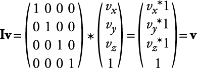
The default model-view and projection matrices are identity matrices. The identity transform is effectively a no-op, as shown in Equation 2-2.

Equation 2-2. Identity transform

Note

For details on how to multiply a vector with a matrix, or a matrix with another matrix, check out the code in the appendix.

It’s important to note that this book uses row vector notation rather than column vector notation. In Equation 2-2, both the left side of (vx vy vz 1) and right side of (vx*1 vy*1 vz*1 1) are 4D row vectors. That equation could, however, be expressed in column vector notation like so:

Sometimes it helps to think of a 4D row vector as being a 1×4 matrix, and a 4D column vector as being a 4×1 matrix. (nxm denotes the dimensions of a matrix where n is the number of rows and m is the number of columns.)

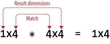
Figure 2-6 shows a trick for figuring out whether it’s legal to multiply two quantities in a certain order: the inner numbers should match. The outer numbers tell you the dimensions of the result. Applying this rule, we can see that it’s legal to multiply the two matrices shown in Equation 2-2: the 4D row vector (effectively a 1×4 matrix) on the left of the * and the 4×4 matrix on the right are multiplied to produce a 1×4 matrix (which also happens to be a 4D row vector).

Figure 2-6. Matrix multiplication dimensionality

From a coding perspective, I find that row vectors are more natural than column vectors because they look like tiny C-style arrays. It’s valid to think of them as column vectors if you’d like, but if you do so, be aware that the ordering of your transforms will flip around. Ordering is crucial because matrix multiplication is not commutative.

Consider this snippet of ES 1.1 code:

glLoadIdentity();
glMultMatrix(A);
glMultMatrix(B);
glMultMatrix(C);
glDrawArrays(...);

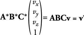
With row vectors, you can think of each successive transform as being premultiplied with the current transform, so the previous snippet is equivalent to the following:

With column vectors, each successive transform is postmultiplied, so the code snippet is actually equivalent to the following:

Regardless of whether you prefer row or column vectors, you should always think of the last transformation in your code as being the first one to be applied to the vertex. To make this apparent with column vectors, use parentheses to show the order of operations:

This illustrates another reason why I like row vectors; they make OpenGL’s reverse-ordering characteristic a little more obvious.

Enough of this mathematical diversion; let’s get back to the photography metaphor and see how it translates into OpenGL. OpenGL ES 1.1 provides a set of helper functions that can generate a matrix and multiply the current transformation by the result, all in one step. We’ll go over each of these helper functions in the coming sections. Since ES 2.0 does not provide helper functions, we’ll also show what they do behind the scenes so that you can implement them yourself.

Recall that there are three matrices involved in OpenGL’s setup:

1. Adjust the camera’s field-of-view angle; this is the projection matrix.

2. Position the camera and aim it in the appropriate direction; this is the view matrix.

3. Scale, rotate, and translate each object; this is the model matrix.

We’ll go over each of these three transforms in reverse so that we can present the simplest transformations first.

Setting the Model Matrix

The three most common operations when positioning an object in a scene are scale, translation, and rotation.

Scale

The most trivial helper function is glScalef:

float scale[16] = { sx, 0,  0,  0,
                    0,  sy, 0,  0,
                    0,  0,  sz, 0
                    0,  0,  0,  1 };

// The following two statements are equivalent.
glMultMatrixf(scale);
glScalef(sx, sy, sz);

The matrix for scale and its derivation are shown in Equation 2-3.

Equation 2-3. Scale transform

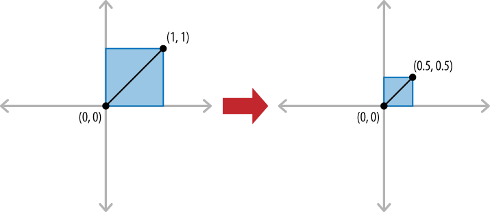
Figure 2-7 depicts a scale transform where s_x = s_y = 0.5.

Figure 2-7. Scale transform

Warning

Nonuniform scale is the case where the x, y, and z scale factors are not all equal to the same value. Such a transformation is perfectly valid, but it can hurt performance in some cases. OpenGL has to do more work to perform the correct lighting computations when nonuniform scale is applied.

Translation

Another simple helper transform is glTranslatef, which shifts an object by a fixed amount:

float translation[16] = { 1,  0,  0,  0,
                          0,  1,  0,  0,
                          0,  0,  1,  0,
                          tx, ty, tz, 1 };

// The following two statements are equivalent.
glMultMatrixf(translation);
glTranslatef(tx, ty, tz);

Intuitively, translation is achieved with addition, but recall that homogeneous coordinates allow us to express all transformations using multiplication, as shown in Equation 2-4.

Equation 2-4. Translation transform

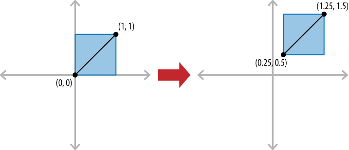
Figure 2-8 depicts a translation transform where t_x = 0.25 and t_y = 0.5.

Rotation

You might recall this transform from the fixed-function variant (ES 1.1) of the HelloArrow sample:

glRotatef(m_currentAngle, 0, 0, 1);

This applies a counterclockwise rotation about the z-axis. The first argument is an angle in degrees; the latter three arguments define the axis of rotation. The ES 2.0 renderer in HelloArrow was a bit tedious because it computed the matrix manually:

#include <cmath>
...
float radians = m_currentAngle * Pi / 180.0f;
float s = std::sin(radians);
float c = std::cos(radians);
float zRotation[16] = { c, s, 0, 0,
                       -s, c, 0, 0,
                        0, 0, 1, 0,
                        0, 0, 0, 1 };

GLint modelviewUniform = glGetUniformLocation(m_simpleProgram, "Modelview");
glUniformMatrix4fv(modelviewUniform, 1, 0, &zRotation[0]);

Figure 2-8. Translation transform

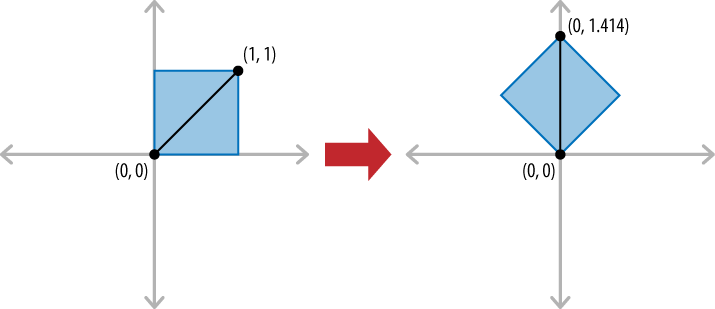
Figure 2-9 depicts a rotation transform where the angle is 45°.

Figure 2-9. Rotation transform

Rotation about the z-axis is relatively simple, but rotation around an arbitrary axis requires a more complex matrix. For ES 1.1, glRotatef generates the matrix for you, so there’s no need to get too concerned with its contents. For ES 2.0, check out the appendix to see how to implement this.

By itself, glRotatef rotates only around the origin, so what if you want to rotate around an arbitrary point p? To accomplish this, use a three-step process:

1. Translate by -p.

2. Perform the rotation.

3. Translate by +p.

For example, to change HelloArrow to rotate around (0, 1) rather than the center, you could do this:

glTranslatef(0, +1, 0);
glRotatef(m_currentAngle, 0, 0, 1);
glTranslatef(0, -1, 0);
glDrawArrays(...);

Remember, the last transform in your code is actually the first one that gets applied!

Setting the View Transform

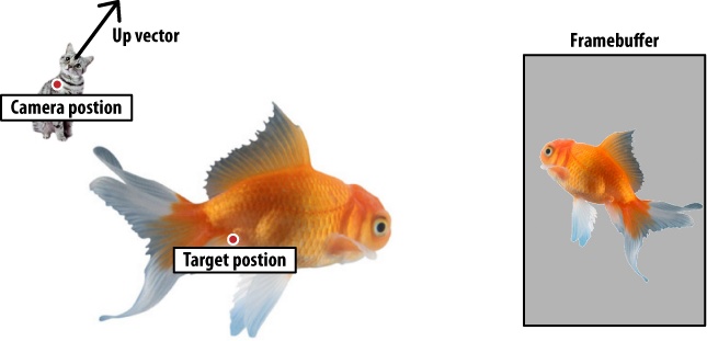
The simplest way to create a view matrix is with the popular LookAt function. It’s not built into OpenGL ES, but it’s easy enough to implement it from scratch. LookAt takes three parameters: a camera position, a target location, and an “up” vector to define the camera’s orientation (see Figure 2-10).

Using the three input vectors, LookAt produces a transformation matrix that would otherwise be cumbersome to derive using the fundamental transforms (scale, translation, rotation). Example 2-1 is one possible implementation of LookAt.

Example 2-1. LookAt

mat4 LookAt(const vec3& eye, const vec3& target, const vec3& up)
{
    vec3 z = (eye - target).Normalized();
    vec3 x = up.Cross(z).Normalized();
    vec3 y = z.Cross(x).Normalized();

    mat4 m;
    m.x = vec4(x, 0);
    m.y = vec4(y, 0);
    m.z = vec4(z, 0);
    m.w = vec4(0, 0, 0, 1);

    vec4 eyePrime = m * -eye;
    m = m.Transposed();
    m.w = eyePrime;

    return m;
}

Figure 2-10. The LookAt transform

Note that Example 2-1 uses custom types like vec3, vec4, and mat4. This isn’t pseudocode; it’s actual code from the C++ vector library in the appendix. We’ll discuss the library later in the chapter.

Setting the Projection Transform

Until this point, we’ve been dealing with transformations that are typically used to modify the model-view rather than the projection. ES 1.1 operations such as glRotatef and glTranslatef always affect the current matrix, which can be changed at any time using glMatrixMode. Initially the matrix mode is GL_MODELVIEW.

What’s the distinction between projection and model-view? Novice OpenGL programmers sometimes think of the projection as being the “camera matrix,” but this is an oversimplification, if not completely wrong; the position and orientation of the camera should actually be specified in the model-view. I prefer to think of the projection as being the camera’s “zoom lens” because it affects the field of view.

Warning

Camera position and orientation should always go in the model-view, not the projection. OpenGL ES 1.1 depends on this to perform correct lighting calculations.

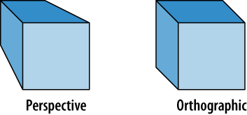
Two types of projections commonly appear in computer graphics: perspective and orthographic. Perspective projections cause distant objects to appear smaller, just as they do in real life. You can see the difference in Figure 2-11.

Figure 2-11. Types of projections

An orthographic projection is usually appropriate only for 2D graphics, so that’s what we used in HelloArrow:

const float maxX = 2;
const float maxY = 3;
glOrthof(-maxX, +maxX, -maxY, +maxY, -1, 1);

The arguments for glOrthof specify the distance of the six bounding planes from the origin: left, right, bottom, top, near, and far. Note that our example arguments create an aspect ratio of 2:3; this is appropriate since the iPhone’s screen is 320×480. The ES 2.0 renderer in HelloArrow reveals how the orthographic projection is computed:

float a = 1.0f / maxX;
float b = 1.0f / maxY;
float ortho[16] = {
    a, 0,  0, 0,
    0, b,  0, 0,
    0, 0, -1, 0,
    0, 0,  0, 1
};

When an orthographic projection is centered around the origin, it’s really just a special case of the scale matrix that we already presented in Scale:

sx = 1.0f / maxX
sy = 1.0f / maxY
sz = -1

float scale[16] = { sx, 0,  0,  0,
                    0,  sy, 0,  0,
                    0,  0,  sz, 0
                    0,  0,  0,  1 };

Since HelloCone (the example you’ll see later in this chapter) will have true 3D rendering, we’ll give it a perspective matrix using the glFrustumf command, like this:

glFrustumf(-1.6f, 1.6, -2.4, 2.4, 5, 10);

The arguments to glFrustumf are the same as glOrthof. Since glFrustum does not exist in ES 2.0, HelloCone’s 2.0 renderer will compute the matrix manually, like this:

void ApplyFrustum(float left, float right, float bottom, 
                  float top, float near, float far)
{
    float a = 2 * near / (right - left);
    float b = 2 * near / (top - bottom);
    float c = (right + left) / (right - left);
    float d = (top + bottom) / (top - bottom);
    float e = - (far + near) / (far - near);
    float f = -2 * far * near / (far - near);

    mat4 m;
    m.x.x = a; m.x.y = 0; m.x.z = 0; m.x.w = 0;
    m.y.x = 0; m.y.y = b; m.y.z = 0; m.y.w = 0;
    m.z.x = c; m.z.y = d; m.z.z = e; m.z.w = -1;
    m.w.x = 0; m.w.y = 0; m.w.z = f; m.w.w = 1;

    glUniformMatrix4fv(projectionUniform, 1, 0, m.Pointer());
}

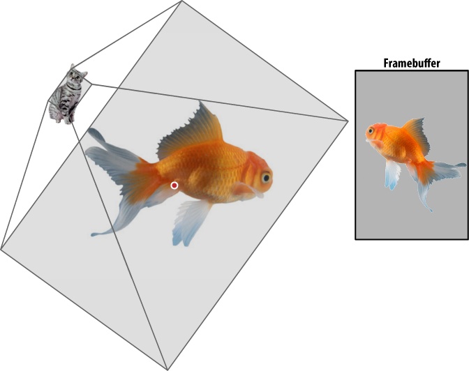
When a perspective projection is applied, the field of view is in the shape of a frustum. The viewing frustum is just a chopped-off pyramid with the eye at the apex of the pyramid (see Figure 2-12).

Figure 2-12. Viewing frustum

A viewing frustum can also be computed based on the angle of the pyramid’s apex (known as field of view); some developers find these to be more intuitive than specifying all six planes. The function in Example 2-2 takes four arguments: the field-of-view angle, the aspect ratio of the pyramid’s base, and the near and far planes.

Example 2-2. VerticalFieldOfView

void VerticalFieldOfView(float degrees, float aspectRatio, 
                         float near, float far)
{
   float top = near * std::tan(degrees * Pi / 360.0f);
   float bottom = -top;
   float left = bottom * aspectRatio;
   float right = top * aspectRatio;

   glFrustum(left, right, bottom, top, near, far);
}

Caution

For perspective projection, avoid setting your near or far plane to zero or a negative number. Mathematically this just doesn’t work out.

Saving and Restoring Transforms with Matrix Stacks

Recall that the ES 1.1 renderer in HelloArrow used glPushMatrix and glPopMatrix to save and restore the transformation state:

void RenderingEngine::Render()
{
    glPushMatrix();
    ...
    glDrawArrays(GL_TRIANGLES, 0, vertexCount);
    ...
    glPopMatrix();
}

It’s fairly standard practice to wrap the Render method in a push/pop block like this, because it prevents transformations from accumulating from one frame to the next.

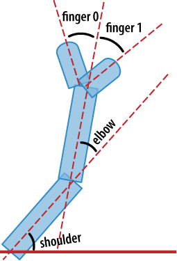
In the previous example, the matrix stack is never more than two entries deep, but the iPhone allows up to 16 stack entries. This facilitates complex sequences of transforms, such as those required to render the articulated arm in Figure 2-13, or any other hierarchical model. When writing code with frequent pushes and pops, it helps to add extra indentation, as in Example 2-3.

Example 2-3. Hierarchical transforms

void DrawRobotArm()
{
    glPushMatrix();
        glRotatef(shoulderAngle, 0, 0, 1);
        glDrawArrays( ... ); // Upper arm
        glTranslatef(upperArmLength, 0, 0);
        glRotatef(elbowAngle, 0, 0, 1);
        glDrawArrays( ... ); // Forearm
        glTranslatef(forearmLength, 0, 0);
        glPushMatrix();
            glRotatef(finger0Angle, 0, 0, 1);
            glDrawArrays( ... ); // Finger 0
        glPopMatrix();
        glPushMatrix();
            glRotatef(-finger1Angle, 0, 0, 1);
            glDrawArrays( ... ); // Finger 1
        glPopMatrix();
    glPopMatrix();
}

Figure 2-13. Robot arm

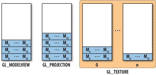
Each matrix mode has its own stack, as depicted in Figure 2-14; typically GL_MODELVIEW gets the heaviest use. Don’t worry about the GL_TEXTURE stacks; we’ll cover them in another chapter. Earlier we mentioned that OpenGL transforms every vertex position by the “current” model-view and projection matrices, by which we meant the topmost element in their respective stacks. To switch from one stack to another, use glMatrixMode.

Figure 2-14. Matrix stacks

Matrix stacks do not exist in ES 2.0; if you need them, you’ll need to create them in your application code or in your own math library. Again, this may seem cruel, but always keep in mind that ES 2.0 is a “closer to the metal” API and that it actually gives you much more power and control through the use of shaders.

Animation

As we’ve seen so far, OpenGL performs quite a bit of math behind the scenes. But ultimately OpenGL is just a low-level graphics API and not an animation API. Luckily, the math required for animation is quite simple.

To sum it up in five words, animation is all about interpolation. An application’s animation system will often take a set of keyframes from an artist, user, or algorithm. At runtime, it computes values between those keyframes. The type of data associated with keyframes can be anything, but typical examples are color, position, and rotation.

Interpolation Techniques

The process of computing an intermediate frame from two keyframes is called tweening. If you divide elapsed time by desired duration, you get a blend weight between zero and one. There are three easing equations discussed here, depicted in Figure 2-15. The tweened value for blending weight t can be computed as follows:

float LinearTween(float t, float start, float end)
{
    return t * start + (1 - t) * end;
}

Certain types of animation should not use linear tweening; a more natural look can often be achieved with one of Robert Penner’s easing equations. Penner’s quadratic ease-in is fairly straightforward:

float QuadraticEaseIn(float t, float start, float end)
{
    return LinearTween(t * t, start, end);
}

Figure 2-15. Easing equations: linear, quadratic ease-in, and quadratic ease-in-out

Penner’s “quadratic ease-in-out” equation is a bit more complex but relatively easy to follow when splitting it into multiple steps, as in Example 2-4.

Example 2-4. Quadratic ease-in-out

float QuadraticEaseInOut(float t, float start, float end)
{
    float middle = (start + end) / 2;
    t = 2 * t;
    if (t <= 1)
        return LinearTween(t * t, start, middle);
    t -= 1;
    return LinearTween(t * t, middle, end);
}

Animating Rotation with Quaternions

For position and color keyframes, it’s easy to perform interpolation: simply call one the aforementioned tweening functions on each of the XYZ or RGB components. At first, rotation seems simple, too; it’s just a matter of tweening the angle. But what if you’re interpolating between two orientations that don’t have the same axis of rotation?

Picture the robot arm example in Figure 2-13. This example was restricted to the plane, but consider what you’d need if each joint were a ball joint. Storing an angle for each joint would be insufficient—you’d also need the axis of rotation. This is known as axis-angle notation and requires a total of four floating-point values for each joint.

It turns out there’s an artful way to represent an arbitrary rotation using the same number of floats as axis-angle, but in a way that often better lends itself to interpolation. This type of 4D vector is called a quaternion, and it was conceived in 1843. Quaternions were somewhat marginalized when modern vector algebra came about, but they experienced a revival in the computer graphics era. Ken Shoemake is one of the people who popularized them in the late 1980s with his famous slerp equation for interpolating between two quaternions.

Warning

Shoemake’s method is actually only one of several methods of quaternion interpolation, but it’s the most popular, and it’s the one we use in our vector library. Other methods, such as normalized quaternion lerp and log-quaternion lerp, are sometimes more desirable in terms of performance.

Having said all this, be aware that quaternions aren’t always the best way to handle an animation problem. Sometimes it suffices to simply compute the angle between two vectors, find an axis of rotation, and interpolate the angle. However, quaternions solve a slightly more complex problem. They don’t merely interpolate between two vectors; they interpolate between two orientations. This may seem pedantic, but it’s an important distinction. Hold your arm straight out in front of you, palm up. Now, bend your arm at the elbow while simultaneously rotating your hand. What you’ve just done is interpolate between two orientations.

It turns out that quaternions are particularly well suited to the type of “trackball” rotation that we’ll be using in much of our sample code. I won’t bore you with a bunch of equations here, but you can check out the appendix to see how to implement quaternions. We’ll leverage this in the HelloCone sample and in the wireframe viewer presented in the next chapter.

Vector Beautification with C++

Recall the vertex structure in HelloArrow:

struct Vertex {
    float Position[2];
    float Color[4];
};

If we kept using vanilla C arrays like this throughout this book, life would become very tedious! What we really want is something like this:

struct Vertex {
    vec2 Position;
    vec4 Color;
};

This is where the power of C++ operator overloading and class templates really shines. It makes it possible (in fact, it makes it easy) to write a small class library that makes much of your application code look like it’s written in a vector-based language. In fact, that’s what we’ve done for the samples in this book. Our entire library consists of only three header files and no .cpp files:

Vector.hpp

Defines a suite of 2D, 3D, and 4D vector types that can be either float-based or integer-based. Has no dependencies on any other header.

Matrix.hpp

Defines classes for 2×2, 3×3, and 4×4 matrices. Depends only on Vector.hpp.

Quaternion.hpp

Defines a class for quaternions and provides several methods for interpolation and construction. Depends on Matrix.hpp.

These files are listed in their entirety in the appendix, but to give you a taste of how the library is structured, Example 2-5 shows portions of Vector.hpp.

Example 2-5. Vector.hpp

#pragma once
#include <cmath>

template <typename T>
struct Vector2 {
    Vector2() {}
    Vector2(T x, T y) : x(x), y(y) {}
    T x;
    T y;
    ...
};

template <typename T>
struct Vector3 {
    Vector3() {}
    Vector3(T x, T y, T z) : x(x), y(y), z(z) {}
    void Normalize()
    {
        float length = std::sqrt(x * x + y * y + z * z);
        x /= length;
        y /= length;
        z /= length;
    }
    Vector3 Normalized() const 
    {
        Vector3 v = *this;
        v.Normalize();
        return v;
    }
    Vector3 Cross(const Vector3& v) const
    {
        return Vector3(y * v.z - z * v.y,
                       z * v.x - x * v.z,
                       x * v.y - y * v.x);
    }
    T Dot(const Vector3& v) const
    {
        return x * v.x + y * v.y + z * v.z;
    }
    Vector3 operator-() const
    {
        return Vector3(-x, -y, -z);
    }
    bool operator==(const Vector3& v) const
    {
        return x == v.x && y == v.y && z == v.z;
    }
    T x;
    T y;
    T z;
};

template <typename T>
struct Vector4 {
    ...
};

typedef Vector2<int> ivec2;
typedef Vector3<int> ivec3;
typedef Vector4<int> ivec4;

typedef Vector2<float> vec2;
typedef Vector3<float> vec3;
typedef Vector4<float> vec4;

Note how we parameterized each vector type using C++ templates. This allows the same logic to be used for both float-based vectors and integer-based vectors.

Even though a 2D vector has much in common with a 3D vector, we chose not to share logic between them. This could’ve been achieved by adding a second template argument for dimensionality, as in the following:

template <typename T, int Dimension>
struct Vector {
    ...
    T components[Dimension];
};

When designing a vector library, it’s important to strike the right balance between generality and readability. Since there’s relatively little logic in each vector class and since we rarely need to iterate over vector components, defining separate classes seems like a reasonable way to go. It’s also easier for readers to understand the meaning of, say, Position.y than Position[1].

Since a good bit of application code will be making frequent use of these types, the bottom of Example 2-5 defines some abbreviated names using typedefs. Lowercase names such as vec2 and ivec4 break the naming convention we’ve established for types, but they adopt a look and feel similar to native types in the language itself.

The vec2/ivec2 style names in our C++ vector library are directly pilfered from keywords in GLSL. Take care not to confuse this book’s C++ listings with shader listings.

Warning

In GLSL shaders, types such as vec2 and mat4 are built into the language itself. Our C++ vector library merely mimics them.

HelloCone with Fixed Function

We’re finally ready to upgrade the HelloArrow program into HelloCone. We’ll not go only from rendering in 2D to rendering in 3D; we’ll also support two new orientations for when the device is held face up or face down.

Even though the visual changes are significant, they’ll all occur within RenderingEngine1.cpp and RenderingEngine2.cpp. That’s the beauty of the layered, interface-based approach presented in the previous chapter. First we’ll deal exclusively with the ES 1.1 renderer, RenderingEngine1.cpp.

RenderingEngine Declaration

The implementations of HelloArrow and HelloCone diverge in several ways, as shown in Table 2-5.

Table 2-5. Differences between HelloArrow and HelloCone

HelloArrow	HelloCone
Rotation state is an angle on the z-axis.	Rotation state is a quaternion.
One draw call.	Two draw calls: one for the disk, one for the cone.
Vectors are represented with small C arrays.	Vectors are represented with objects like vec3.
Triangle data is small enough to be hardcoded within the program.	Triangle data is generated at runtime.
Triangle data is stored in a C array.	Triangle data is stored in an STL vector.

STL: To Use or Not to Use?

I decided to use the C++ Standard Template Library (STL) in much of this book’s sample code. The STL simplifies many tasks by providing classes for commonly used data structures, such as resizeable arrays (std::vector) and doubly linked lists (std::list). Many developers would argue against using STL on a mobile platform like the iPhone when writing performance-critical code. It’s true that sloppy usage of STL can cause your application’s memory footprint to get out of hand, but nowadays, C++ compilers do a great job at optimizing STL code. Keep in mind that the iPhone SDK provides a rich set of Objective-C classes (e.g., NSDictionary) that are analogous to many of the STL classes, and they have similar costs in terms of memory footprint and performance.

With Table 2-5 in mind, take a look at the top of RenderingEngine1.cpp, shown in Example 2-6 (note that this moves the definition of struct Vertex higher up in the file than it was before, so you’ll need to remove the old version of this struct from this file).

Note

If you’d like to follow along in code as you read, make a copy of the HelloArrow project folder in Finder, and save it as HelloCone. Open the project in Xcode, and then select Rename from the Project menu. Change the project name to HelloCone, and click Rename. Next, visit the appendix, and add Vector.hpp, Matrix.hpp, and Quaternion.hpp to the project. RenderingEngine1.cpp will be almost completely different, so open it and remove all its content. Now you’re ready to make the changes shown in this section as you read along.

Example 2-6. RenderingEngine1 class declaration

#include <OpenGLES/ES1/gl.h>
#include <OpenGLES/ES1/glext.h>
#include "IRenderingEngine.hpp"
#include "Quaternion.hpp"
#include <vector>

static const float AnimationDuration = 0.25f;

using namespace std;

struct Vertex {
    vec3 Position;
    vec4 Color;
};

struct Animation {
    Quaternion Start;
    Quaternion End;
    Quaternion Current;
    float Elapsed;
    float Duration;
};

class RenderingEngine1 : public IRenderingEngine {
public:
    RenderingEngine1();
    void Initialize(int width, int height);
    void Render() const;
    void UpdateAnimation(float timeStep);
    void OnRotate(DeviceOrientation newOrientation);
private:
    vector<Vertex> m_cone;
    vector<Vertex> m_disk;
    Animation m_animation;
    GLuint m_framebuffer;
    GLuint m_colorRenderbuffer;
    GLuint m_depthRenderbuffer;
};

The Animation structure enables smooth 3D transitions. It includes quaternions for three orientations: the starting orientation, the current interpolated orientation, and the ending orientation. It also includes two time spans: Elapsed and Duration, both of which are in seconds. They’ll be used to compute a slerp fraction between 0 and 1.

The triangle data lives in two STL containers, m_cone and m_disk. The vector container is ideal because we know how big it needs to be ahead of time, and it guarantees contiguous storage. Contiguous storage of vertices is an absolute requirement for OpenGL.

Unlike HelloArrow, there are two renderbuffers here. HelloArrow was 2D and therefore only required a color renderbuffer. HelloCone requires an additional renderbuff for depth. We’ll learn more about the depth buffer in a future chapter; briefly, it’s a special image plane that stores a single Z value at each pixel.

OpenGL Initialization and Cone Tessellation

The construction methods are very similar to what we had in HelloArrow:

IRenderingEngine* CreateRenderer1()
{
    return new RenderingEngine1();
}

RenderingEngine1::RenderingEngine1()
{
    // Create & bind the color buffer so that the caller can allocate its space.
    glGenRenderbuffersOES(1, &m_colorRenderbuffer);
    glBindRenderbufferOES(GL_RENDERBUFFER_OES, m_colorRenderbuffer);
}

The Initialize method, shown in Example 2-7, is responsible for generating the vertex data and setting up the framebuffer. It starts off by defining some values for the cone’s radius, height, and geometric level of detail. The level of detail is represented by the number of vertical “slices” that constitute the cone. After generating all the vertices, it initializes OpenGL’s framebuffer object and transform state. It also enables depth testing since this a true 3D app. We’ll learn more about depth testing in Chapter 4.

Example 2-7. RenderingEngine initialization

void RenderingEngine1::Initialize(int width, int height)
{
    const float coneRadius = 0.5f;
    const float coneHeight = 1.866f;
    const int coneSlices = 40;

    {
      // Generate vertices for the disk.
      ...
    } 

    {
      // Generate vertices for the body of the cone.
      ...
    }

    // Create the depth buffer.
    glGenRenderbuffersOES(1, &m_depthRenderbuffer);
    glBindRenderbufferOES(GL_RENDERBUFFER_OES, m_depthRenderbuffer);
    glRenderbufferStorageOES(GL_RENDERBUFFER_OES,
                             GL_DEPTH_COMPONENT16_OES,
                             width,
                             height);
    
    // Create the framebuffer object; attach the depth and color buffers.
    glGenFramebuffersOES(1, &m_framebuffer);
    glBindFramebufferOES(GL_FRAMEBUFFER_OES, m_framebuffer);
    glFramebufferRenderbufferOES(GL_FRAMEBUFFER_OES,
                                 GL_COLOR_ATTACHMENT0_OES,
                                 GL_RENDERBUFFER_OES,
                                 m_colorRenderbuffer);
    glFramebufferRenderbufferOES(GL_FRAMEBUFFER_OES,
                                 GL_DEPTH_ATTACHMENT_OES,
                                 GL_RENDERBUFFER_OES,
                                 m_depthRenderbuffer);
    
    // Bind the color buffer for rendering.
    glBindRenderbufferOES(GL_RENDERBUFFER_OES, m_colorRenderbuffer);
    
    glViewport(0, 0, width, height);
    glEnable(GL_DEPTH_TEST);
    
    glMatrixMode(GL_PROJECTION);
    glFrustumf(-1.6f, 1.6, -2.4, 2.4, 5, 10);
    
    glMatrixMode(GL_MODELVIEW);
    glTranslatef(0, 0, -7);
}

Much of Example 2-7 is standard procedure when setting up an OpenGL context, and much of it will become clearer in future chapters. For now, here’s a brief summary:

Define some constants to use when generating the vertices for the disk and cone.

Generate an ID for the depth renderbuffer, bind it, and allocate storage for it. We’ll learn more about depth buffers later.

Generate an ID for the framebuffer object, bind it, and attach depth and color to it using glFramebufferRenderbufferOES.

Bind the color renderbuffer so that future rendering operations will affect it.

Set up the left, bottom, width, and height properties of the viewport.

Turn on depth testing since this is a 3D scene.

Set up the projection and model-view transforms.

Example 2-7 replaces the two pieces of vertex generation code with ellipses because they deserve an in-depth explanation. The problem of decomposing an object into triangles is called triangulation, but more commonly you’ll see the term tessellation, which actually refers to the broader problem of filling a surface with polygons. Tessellation can be a fun puzzle, as any M.C. Escher fan knows; we’ll learn more about it in later chapters.

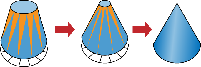
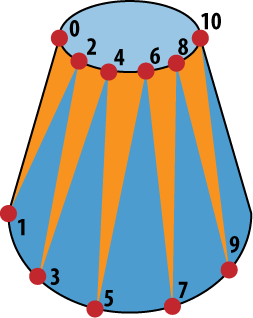
For now let’s form the body of the cone with a triangle strip and the bottom cap with a triangle fan, as shown in Figure 2-16.

Figure 2-16. Tessellation in HelloCone

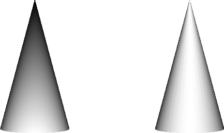
To form the shape of the cone’s body, we could use a fan rather than a strip, but this would look strange because the color at the fan’s center would be indeterminate. Even if we pick an arbitrary color for the center, an incorrect vertical gradient would result, as shown on the left in Figure 2-17.

Figure 2-17. Left: Cone with triangle fan. Right: Cone with triangle strip

Using a strip for the cone isn’t perfect either because every other triangle is degenerate (shown in gray in Figure 2-16). The only way to fix this would be resorting to GL_TRIANGLES, which requires twice as many elements in the vertex array. It turns out that OpenGL provides an indexing mechanism to help with situations like this, which we’ll learn about in the next chapter. For now we’ll use GL_TRIANGLE_STRIP and live with the degenerate triangles. The code for generating the cone vertices is shown in Example 2-8 and depicted visually in Figure 2-18 (this code goes after the comment // Generate vertices for the body of the cone in RenderingEngine1::Initialize). Two vertices are required for each slice (one for the apex, one for the rim), and an extra slice is required to close the loop (Figure 2-18). The total number of vertices is therefore (n+1)*2 where n is the number of slices. Computing the points along the rim is the classic graphics algorithm for drawing a circle and may look familiar if you remember your trigonometry.

Figure 2-18. Vertex order in HelloCone

Example 2-8. Generation of cone vertices

m_cone.resize((coneSlices + 1) * 2);

// Initialize the vertices of the triangle strip.
vector<Vertex>::iterator vertex = m_cone.begin();
const float dtheta = TwoPi / coneSlices;
for (float theta = 0; vertex != m_cone.end(); theta += dtheta) {
    
    // Grayscale gradient
    float brightness = abs(sin(theta));
    vec4 color(brightness, brightness, brightness, 1);
    
    // Apex vertex
    vertex->Position = vec3(0, 1, 0);
    vertex->Color = color;
    vertex++;
    
    // Rim vertex
    vertex->Position.x = coneRadius * cos(theta);
    vertex->Position.y = 1 - coneHeight;
    vertex->Position.z = coneRadius * sin(theta);
    vertex->Color = color;
    vertex++;
}

Note that we’re creating a grayscale gradient as a cheap way to simulate lighting:

float brightness = abs(sin(theta));
vec4 color(brightness, brightness, brightness, 1);

This is a bit of a hack because the color is fixed and does not change as you reorient the object, but it’s good enough for our purposes. This technique is sometimes called baked lighting, and we’ll learn more about it in Chapter 9. We’ll also learn how to achieve more realistic lighting in Chapter 4.

Example 2-9 generates vertex data for the disk (this code goes after the comment // Generate vertices for the disk in RenderingEngine1::Initialize). Since it uses a triangle fan, the total number of vertices is n+2: one extra vertex for the center, another for closing the loop.

Example 2-9. Generation of disk vertices

// Allocate space for the disk vertices.
m_disk.resize(coneSlices + 2);

// Initialize the center vertex of the triangle fan.
vector<Vertex>::iterator vertex = m_disk.begin();
vertex->Color = vec4(0.75, 0.75, 0.75, 1);
vertex->Position.x = 0;
vertex->Position.y = 1 - coneHeight;
vertex->Position.z = 0;
vertex++;

// Initialize the rim vertices of the triangle fan.
const float dtheta = TwoPi / coneSlices;
for (float theta = 0; vertex != m_disk.end(); theta += dtheta) {
    vertex->Color = vec4(0.75, 0.75, 0.75, 1);
    vertex->Position.x = coneRadius * cos(theta);
    vertex->Position.y = 1 - coneHeight;
    vertex->Position.z = coneRadius * sin(theta);
    vertex++;
}

Smooth Rotation in Three Dimensions

To achieve smooth animation, UpdateAnimation calls Slerp on the rotation quaternion. When a device orientation change occurs, the OnRotate method starts a new animation sequence. Example 2-10 shows these methods.

Example 2-10. UpdateAnimation and OnRotate

void RenderingEngine1::UpdateAnimation(float timeStep)
{
    if (m_animation.Current == m_animation.End)
        return;

    m_animation.Elapsed += timeStep;
    if (m_animation.Elapsed >= AnimationDuration) {
        m_animation.Current = m_animation.End;
    } else {
        float mu = m_animation.Elapsed / AnimationDuration;
        m_animation.Current = m_animation.Start.Slerp(mu, m_animation.End);
    }
}

void RenderingEngine1::OnRotate(DeviceOrientation orientation)
{
    vec3 direction;

    switch (orientation) {
        case DeviceOrientationUnknown:
        case DeviceOrientationPortrait:
            direction = vec3(0, 1, 0);
            break;
            
        case DeviceOrientationPortraitUpsideDown:
            direction = vec3(0, -1, 0);
            break;
            
        case DeviceOrientationFaceDown:       
            direction = vec3(0, 0, -1);
            break;
            
        case DeviceOrientationFaceUp:
            direction = vec3(0, 0, 1);
            break;
            
        case DeviceOrientationLandscapeLeft:
            direction = vec3(+1, 0, 0);
            break;
            
        case DeviceOrientationLandscapeRight:
            direction = vec3(-1, 0, 0);
            break;
    }

    m_animation.Elapsed = 0;
    m_animation.Start = m_animation.Current = m_animation.End;
    m_animation.End = Quaternion::CreateFromVectors(vec3(0, 1, 0), direction);
}

Render Method

Last but not least, HelloCone needs a Render method, as shown in Example 2-11. It’s similar to the Render method in HelloArrow except it makes two draw calls, and the glClear command now has an extra flag for the depth buffer.

Example 2-11. RenderingEngine1::Render

void RenderingEngine1::Render() const
{
    glClearColor(0.5f, 0.5f, 0.5f, 1);
    glClear(GL_COLOR_BUFFER_BIT | GL_DEPTH_BUFFER_BIT);
    glPushMatrix();
    
    glEnableClientState(GL_VERTEX_ARRAY);
    glEnableClientState(GL_COLOR_ARRAY);

    mat4 rotation(m_animation.Current.ToMatrix());
    glMultMatrixf(rotation.Pointer());

    // Draw the cone.
    glVertexPointer(3, GL_FLOAT, sizeof(Vertex), &m_cone[0].Position.x);
    glColorPointer(4, GL_FLOAT, sizeof(Vertex),  &m_cone[0].Color.x);
    glDrawArrays(GL_TRIANGLE_STRIP, 0, m_cone.size());

    // Draw the disk that caps off the base of the cone.
    glVertexPointer(3, GL_FLOAT, sizeof(Vertex), &m_disk[0].Position.x);
    glColorPointer(4, GL_FLOAT, sizeof(Vertex), &m_disk[0].Color.x);
    glDrawArrays(GL_TRIANGLE_FAN, 0, m_disk.size());
    
    glDisableClientState(GL_VERTEX_ARRAY);
    glDisableClientState(GL_COLOR_ARRAY);

    glPopMatrix();
}

Note the call to rotation.Pointer(). In our C++ vector library, vectors and matrices have a method called Pointer(), which exposes a pointer to the first innermost element. This is useful when passing them to OpenGL.

Note

We could’ve made much of our OpenGL code more succinct by changing the vector library such that it provides implicit conversion operators in lieu of Pointer() methods. Personally, I think this would be error prone and would hide too much from the code reader. For similar reasons, STL’s string class requires you to call its c_str() when you want to get a char*.

Because you’ve implemented only the 1.1 renderer so far, you’ll also need to enable the ForceES1 switch at the top of GLView.mm. At this point, you can build and run your first truly 3D iPhone application! To see the two new orientations, try holding the iPhone over your head and at your waist. See Figure 2-19 for screenshots of all six device orientations.

Figure 2-19. Left to right: Portrait, UpsideDown, FaceUp, FaceDown, LandscapeRight, and LandscapeLeft

HelloCone with Shaders

Rather than modify the version of RenderingEngine2.cpp from HelloArrow, it will be more instructive if we can start our ES 2.0 backend by copying the contents of RenderingEngine1.cpp over whatever is already in RenderingEngine2.cpp, with two exceptions: you’ll need to save the BuildShader and BuildProgram methods from the existing RenderingEngine2.cpp from HelloArrow, so copy them somewhere safe for the moment. If you’re following along, do that now, and then you’ll be ready to make some changes to the file. Example 2-12 shows the top part of RenderingEngine2.cpp. New and changed lines are shown in bold. Some sections of unchanged code are shown as ..., so don’t copy this over the existing code in its entirety (just make the changes and additions shown in bold).

Example 2-12. RenderingEngine2 class declaration

#include <OpenGLES/ES2/gl.h>
#include <OpenGLES/ES2/glext.h>
#include "IRenderingEngine.hpp"
#include "Quaternion.hpp"
#include <vector>
#include <iostream>

#define STRINGIFY(A)  #A
#include "../Shaders/Simple.vert"
#include "../Shaders/Simple.frag"

static const float AnimationDuration = 0.25f;

...

class RenderingEngine2 : public IRenderingEngine {
public:
    RenderingEngine2();
    void Initialize(int width, int height);
    void Render() const;
    void UpdateAnimation(float timeStep);
    void OnRotate(DeviceOrientation newOrientation);
private:
    GLuint BuildShader(const char* source, GLenum shaderType) const;
    GLuint BuildProgram(const char* vShader, const char* fShader) const;
    vector<Vertex> m_cone;
    vector<Vertex> m_disk;
    Animation m_animation;
    GLuint m_simpleProgram;
    GLuint m_framebuffer;
    GLuint m_colorRenderbuffer;
    GLuint m_depthRenderbuffer;
};

The Initialize method almost stays as is, but this bit is no longer valid:

    glMatrixMode(GL_PROJECTION);
    glFrustumf(-1.6f, 1.6, -2.4, 2.4, 5, 10);
    
    glMatrixMode(GL_MODELVIEW);
    glTranslatef(0, 0, -7);

For ES 2.0, this changes to the following:

    m_simpleProgram = BuildProgram(SimpleVertexShader, 
                                   SimpleFragmentShader);
    glUseProgram(m_simpleProgram);

    // Set the projection matrix.
    GLint projectionUniform = glGetUniformLocation(m_simpleProgram, 
                                                   "Projection");
    mat4 projectionMatrix = mat4::Frustum(-1.6f, 1.6, -2.4, 2.4, 5, 10);
    glUniformMatrix4fv(projectionUniform, 1, 0, 
                       projectionMatrix.Pointer());

The BuildShader and BuildProgram methods are the same as they were for the ES 2.0 version of HelloArrow; no need to list them here. The shaders themselves are also the same as HelloArrow’s shaders; remember, the lighting is “baked,” so simply passing through the colors is sufficient.

We set up the model-view within the Render method, as shown in Example 2-13. Remember, glUniformMatrix4fv plays a role similar to the glLoadMatrix function in ES 1.1.

Example 2-13. RenderingEngine2::Render

void RenderingEngine2::Render() const
{
    GLuint positionSlot = glGetAttribLocation(m_simpleProgram, 
                                              "Position");
    GLuint colorSlot = glGetAttribLocation(m_simpleProgram, 
                                           "SourceColor");

    glClearColor(0.5f, 0.5f, 0.5f, 1);
    glClear(GL_COLOR_BUFFER_BIT | GL_DEPTH_BUFFER_BIT);
    
    glEnableVertexAttribArray(positionSlot);
    glEnableVertexAttribArray(colorSlot);
    
    mat4 rotation(m_animation.Current.ToMatrix());
    mat4 translation = mat4::Translate(0, 0, -7);

    // Set the model-view matrix.
    GLint modelviewUniform = glGetUniformLocation(m_simpleProgram, 
                                                  "Modelview");
    mat4 modelviewMatrix = rotation * translation;
    glUniformMatrix4fv(modelviewUniform, 1, 0, modelviewMatrix.Pointer());
    
    // Draw the cone.
    {
      GLsizei stride = sizeof(Vertex);
      const GLvoid* pCoords = &m_cone[0].Position.x;
      const GLvoid* pColors = &m_cone[0].Color.x;
      glVertexAttribPointer(positionSlot, 3, GL_FLOAT, 
                            GL_FALSE, stride, pCoords);
      glVertexAttribPointer(colorSlot, 4, GL_FLOAT, 
                            GL_FALSE, stride, pColors);
      glDrawArrays(GL_TRIANGLE_STRIP, 0, m_cone.size());
    }
    
    // Draw the disk that caps off the base of the cone.
    {
      GLsizei stride = sizeof(Vertex);
      const GLvoid* pCoords = &m_disk[0].Position.x;
      const GLvoid* pColors = &m_disk[0].Color.x;
      glVertexAttribPointer(positionSlot, 3, GL_FLOAT, 
                            GL_FALSE, stride, pCoords);
      glVertexAttribPointer(colorSlot, 4, GL_FLOAT, 
                            GL_FALSE, stride, pColors);
      glDrawArrays(GL_TRIANGLE_FAN, 0, m_disk.size());
    }
    
    glDisableVertexAttribArray(positionSlot);
    glDisableVertexAttribArray(colorSlot);
}

The sequence of events in Example 2-13 is actually quite similar to the sequence in Example 2-11; only the details have changed.

Next, go through the file, and change any remaining occurrences of RenderingEngine1 to RenderingEngine2, including the factory method (and be sure to change the name of that method to CreateRenderer2). You also need to remove any occurrences of _OES and OES. Now, turn off the ForceES1 switch in GLView.mm; this completes the changes required for the shader-based version of HelloCone. It may seem silly to have added an ES 2.0 renderer without having added any cool shader effects, but it illustrates the differences between the two APIs.

Wrapping Up

This chapter was perhaps the most academic part of this book, but we disseminated some fundamental graphics concepts and cleared up some of the sample code that was glossed over in the first chapter.

Understanding transforms is perhaps the most difficult but also the most crucial hurdle to overcome for OpenGL newbies. I encourage you to experiment with HelloCone to get a better feel for how transformations work. For example, try adding some hard-coded rotations and translations to the Render method, and observe how their ordering affects the final rendering.

In the next chapter, you’ll learn more about submitting geometry to OpenGL, and you’ll get a primer on the iPhone’s touchscreen.