iPhone 3D Programming

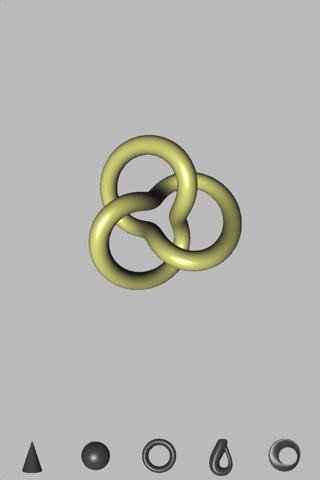
Chapter 4. Adding Depth and Realism

Lumos!

—Harry Potter and the Chamber of Secrets, J.K. Rowling

When my wife and I go out to see a film packed with special effects, I always insist on sitting through the entire end credits, much to her annoyance. It never ceases to amaze me how many artists work together to produce a Hollywood blockbuster. I’m often impressed with the number of artists whose full-time job concerns lighting. In Pixar’s Up, at least five people have the title “lighting technical director,” four people have the title “key lighting artist,” and another four people have the honor of “master lighting artist.”

Lighting is obviously a key aspect to understanding realism in computer graphics, and that’s much of what this chapter is all about. We’ll refurbish the wireframe viewer sample to use lighting and triangles, rechristening it to Model Viewer. We’ll also throw some light on the subject of shaders, which we’ve been glossing over until now (in ES 2.0, shaders are critical to lighting). Finally, we’ll further enhance the viewer app by giving it the ability to load model files so that we’re not stuck with parametric surfaces forever. Mathematical shapes are great for geeking out, but they’re pretty lame for impressing your 10-year-old!

Examining the Depth Buffer

Before diving into lighting, let’s take a closer look at depth buffers, since we’ll need to add one to wireframe viewer. You might recall the funky framebuffer object (FBO) setup code in the HelloCone sample presented in Example 2-7, repeated here in Example 4-1.

Example 4-1. Depth buffer setup

// Create the depth buffer.
glGenRenderbuffersOES(1, &m_depthRenderbuffer);
glBindRenderbufferOES(GL_RENDERBUFFER_OES, m_depthRenderbuffer);
glRenderbufferStorageOES(GL_RENDERBUFFER_OES,
                         GL_DEPTH_COMPONENT16_OES,
                         width,
                         height);
    
// Create the framebuffer object; attach the depth and color buffers.
glGenFramebuffersOES(1, &m_framebuffer);
glBindFramebufferOES(GL_FRAMEBUFFER_OES, m_framebuffer);
glFramebufferRenderbufferOES(GL_FRAMEBUFFER_OES,
                             GL_COLOR_ATTACHMENT0_OES,
                             GL_RENDERBUFFER_OES,
                             m_colorRenderbuffer);
glFramebufferRenderbufferOES(GL_FRAMEBUFFER_OES,
                             GL_DEPTH_ATTACHMENT_OES,
                             GL_RENDERBUFFER_OES,
                             m_depthRenderbuffer);
    
// Bind the color buffer for rendering.
glBindRenderbufferOES(GL_RENDERBUFFER_OES, m_colorRenderbuffer);

glViewport(0, 0, width, height);
glEnable(GL_DEPTH_TEST);

...

Create a handle to the renderbuffer object that stores depth.

Bind the newly created handle, making it affected by subsequent renderbuffer commands.

Allocate storage for the depth buffer using 16-bit precision.

Attach the depth buffer to the framebuffer object.

Enable depth testing—we’ll explain this shortly.

Why does HelloCone need a depth buffer when wireframe viewer does not? When the scene is composed of nothing but monochrome lines, we don’t care about the visibility problem; this means we don’t care which lines are obscured by other lines. HelloCone uses triangles rather than lines, so the visibility problem needs to be addressed. OpenGL uses the depth buffer to handle this problem efficiently.

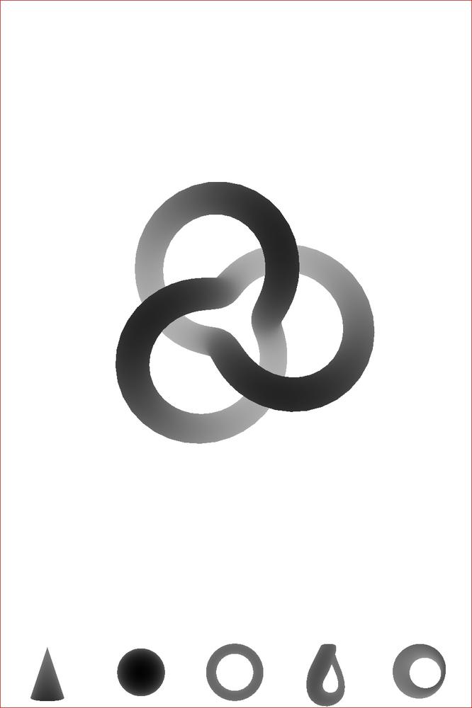
Figure 4-1 depicts ModelViewer’s depth buffer in grayscale: white pixels are far away, black pixels are nearby. Even though users can’t see the depth buffer, OpenGL needs it for its rendering algorithm. If it didn’t have a depth buffer, you’d be forced to carefully order your draw calls from farthest to nearest. (Incidentally, such an ordering is called the painter’s algorithm, and there are special cases where you’ll need to use it anyway, as you’ll see in Blending Caveats.)

Figure 4-1. Depth buffer in ModelViewer

OpenGL uses a technique called depth testing to solve the visibility problem. Suppose you were to render a red triangle directly in front of the camera and then draw a green triangle directly behind the red triangle. Even though the green triangle is drawn last, you’d want to the red triangle to be visible; the green triangle is said to be occluded. Here’s how it works: every rasterized pixel not only has its RGB values written to the color buffer but also has its Z value written to the depth buffer. OpenGL “rejects” occluded pixels by checking whether their Z value is greater than the Z value that’s already in the depth buffer. In pseudocode, the algorithm looks like this:

void WritePixel(x, y, z, color)
{
    if (DepthTestDisabled || z < DepthBuffer[x, y]) {
        DepthBuffer[x, y] = z;
        ColorBuffer[x, y] = color;
    }
}

Beware the Scourge of Depth Artifacts

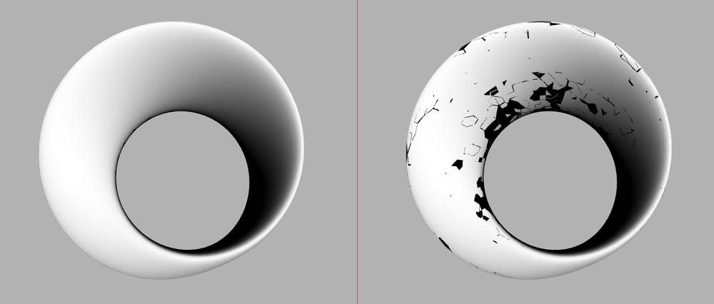
Something to watch out for with depth buffers is Z-fighting, which is a visual artifact that occurs when overlapping triangles have depths that are too close to each other (see Figure 4-2).

Figure 4-2. Z-fighting in the Möbius strip

Recall that the projection matrix defines a viewing frustum bounded by six planes (Setting the Projection Transform). The two planes that are perpendicular to the viewing direction are called the near plane and far plane. In ES 1.1, these planes are arguments to the glOrtho or glPerspective functions; in ES 2.0, they’re passed to a custom function like the mat4::Frustum method in the C++ vector library from the appendix.

It turns out that if the near plane is too close to the camera or if the far plane is too distant, this can cause precision issues that result in Z-fighting. However this is only one possible cause for Z-fighting; there are many more. Take a look at the following list of suggestions if you ever see artifacts like the ones in Figure 4-2.

Push out your near plane.

For perspective projections, having the near plane close to zero can be detrimental to precision.

Pull in your far plane.

Similarly, the far plane should still be pulled in as far as possible without clipping away portions of your scene.

Scale your scene smaller.

Try to avoid defining an astronomical-scale scene with huge extents.

Increase the bit width of your depth buffer.

All iPhones and iPod touches (at the time of this writing) support 16-bit and 24-bit depth formats. The bit width is determined according to the argument you pass to glRenderbufferStorageOES when allocating the depth buffer.

Are you accidentally rendering coplanar triangles?

The fault might not lie with OpenGL but with your application code. Perhaps your generated vertices are lying on the same Z plane because of a rounding error.

Do you really need depth testing in the first place?

In some cases you should probably disable depth testing anyway. For example, you don’t need it if you’re rendering a 2D heads-up display. Disabling the depth test can also boost performance.

Creating and Using the Depth Buffer

Let’s enhance the wireframe viewer by adding in a depth buffer; this paves the way for converting the wireframes into solid triangles. Before making any changes, use Finder to make a copy of the folder that contains the SimpleWireframe project. Rename the folder to ModelViewer, and then open the copy of the SimpleWireframe project inside that folder. Select Project→Rename, and rename the project to ModelViewer.

Open RenderingEngine.ES1.cpp, and add GLuint m_depthRenderbuffer; to the private: section of the class declaration. Next, find the Initialize method, and delete everything from the comment // Create the framebuffer object to the glBindRenderbufferOES call. Replace the code you deleted with the code in Example 4-2.

Example 4-2. Adding depth to ES1::RenderingEngine::Initialize

// Extract width and height from the color buffer.
int width, height;
glGetRenderbufferParameterivOES(GL_RENDERBUFFER_OES,
                                GL_RENDERBUFFER_WIDTH_OES, &width);
glGetRenderbufferParameterivOES(GL_RENDERBUFFER_OES,
                                GL_RENDERBUFFER_HEIGHT_OES, &height);

// Create a depth buffer that has the same size as the color buffer.
glGenRenderbuffersOES(1, &m_depthRenderbuffer);
glBindRenderbufferOES(GL_RENDERBUFFER_OES, m_depthRenderbuffer);
glRenderbufferStorageOES(GL_RENDERBUFFER_OES, GL_DEPTH_COMPONENT16_OES,
                         width, height);

// Create the framebuffer object.
GLuint framebuffer;
glGenFramebuffersOES(1, &framebuffer);
glBindFramebufferOES(GL_FRAMEBUFFER_OES, framebuffer);
glFramebufferRenderbufferOES(GL_FRAMEBUFFER_OES, GL_COLOR_ATTACHMENT0_OES,
                             GL_RENDERBUFFER_OES, m_colorRenderbuffer);
glFramebufferRenderbufferOES(GL_FRAMEBUFFER_OES, GL_DEPTH_ATTACHMENT_OES,
                             GL_RENDERBUFFER_OES, m_depthRenderbuffer);
glBindRenderbufferOES(GL_RENDERBUFFER_OES, m_colorRenderbuffer);

// Enable depth testing.
glEnable(GL_DEPTH_TEST);

The ES 2.0 variant of Example 4-2 is almost exactly the same. Repeat the process in that file, but remove all _OES and OES suffixes.

Next, find the call to glClear (in both rendering engines), and add a flag for depth:

glClear(GL_COLOR_BUFFER_BIT | GL_DEPTH_BUFFER_BIT);

At this point, you should be able to compile and run, although depth testing doesn’t buy you anything yet since the app is still rendering in wireframe.

By default, the depth buffer gets cleared to a value of 1.0; this makes sense since you want all your pixels to initially pass the depth test, and OpenGL clamps the maximum window-space Z coordinate to 1.0. Incidentally, if you want to clear the depth buffer to some other value, you can call glClearDepthf, similar to glClearColor. You can even configure the depth test itself using glDepthFunc. By default, pixels “win” if their Z is less than the value in the depth buffer, but you can change the test to any of these conditions:

GL_NEVER

Pixels never pass the depth test.

GL_ALWAYS

Pixels always pass the depth test.

GL_LESS

Pixels pass only if their Z value is less than the Z value in the depth buffer. This is the default.

GL_LEQUAL

Pixels pass only if their Z value is less than or equal to the Z value in the depth buffer.

GL_EQUAL

Pixels pass only if their Z value is equal to the Z value in the depth buffer. This could be used to create an infinitely thin slice of the scene.

GL_GREATER

Pixels pass only if their Z value is greater than the Z value in the depth buffer.

GL_GEQUAL

Pixels pass only if their Z value is greater than or equal to the Z value in the depth buffer.

GL_NOTEQUAL

Pixels pass only if their Z value is not equal to the Z value in the depth buffer.

The flexibility of glDepthFunc is a shining example of how OpenGL is often configurable to an extent more than you really need. I personally admire this type of design philosophy in an API; anything that is reasonably easy to implement in hardware is exposed to the developer at a low level. This makes the API forward-looking because it enables developers to dream up unusual effects that the API designers did not necessarily anticipate.

Filling the Wireframe with Triangles

In this section we’ll walk through the steps required to render parametric surfaces with triangles rather than lines. First we need to enhance the ISurface interface to support the generation of indices for triangles rather than lines. Open Interfaces.hpp, and make the changes shown in bold in Example 4-3.

Example 4-3. Enhanced ISurface interface

struct ISurface {
    virtual int GetVertexCount() const = 0;
    virtual int GetLineIndexCount() const = 0;
    virtual int GetTriangleIndexCount() const = 0;
    virtual void GenerateVertices(vector<float>& vertices) const = 0;
    virtual void GenerateLineIndices(vector<unsigned short>& indices) const = 0;
    virtual void
      GenerateTriangleIndices(vector<unsigned short>& indices) const = 0;
    virtual ~ISurface() {}
};

You’ll also need to open ParametricSurface.hpp and make the complementary changes to the class declaration of ParametricSurface shown in Example 4-4.

Example 4-4. Enhanced ParametricSurface interface

class ParametricSurface : public ISurface {
public:
    int GetVertexCount() const;
    int GetLineIndexCount() const;
    int GetTriangleIndexCount() const;
    void GenerateVertices(vector<float>& vertices) const;
    void GenerateLineIndices(vector<unsigned short>& indices) const;
    void GenerateTriangleIndices(vector<unsigned short>& indices) const;

Next open ParametericSurface.cpp, and add the implementation of GetTriangleIndexCount and GenerateTriangleIndices per Example 4-5.

Example 4-5. ParametricSurface::GenerateTriangleIndices

int ParametricSurface::GetTriangleIndexCount() const
{
    return 6 * m_slices.x * m_slices.y;
}

void
ParametricSurface::GenerateTriangleIndices(vector<unsigned short>& indices) const
{
    indices.resize(GetTriangleIndexCount());
    vector<unsigned short>::iterator index = indices.begin();
    for (int j = 0, vertex = 0; j < m_slices.y; j++) {
        for (int i = 0; i < m_slices.x; i++) {
            int next = (i + 1) % m_divisions.x;
            *index++ = vertex + i;
            *index++ = vertex + next;
            *index++ = vertex + i + m_divisions.x;
            *index++ = vertex + next;
            *index++ = vertex + next + m_divisions.x;
            *index++ = vertex + i + m_divisions.x;
        }
        vertex += m_divisions.x;
    }
}

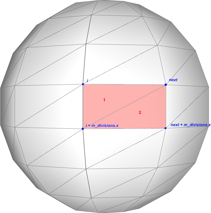
Example 4-5 is computing indices for two triangles, as shown in Figure 4-3.

Figure 4-3. Generating triangle indices for a parametric surface

Now we need to modify the rendering engine so that it calls these new methods when generating VBOs, as in Example 4-6. The modified lines are shown in bold. Make these changes to both RenderingEngine.ES1.cpp and RenderingEngine.ES2.cpp.

Example 4-6. RenderingEngine Modifications for triangles

void RenderingEngine::Initialize(const vector<ISurface*>& surfaces)
{
    vector<ISurface*>::const_iterator surface;
    for (surface = surfaces.begin(); surface != surfaces.end(); ++surface) {
        
        // Create the VBO for the vertices.
        vector<float> vertices;
        (*surface)->GenerateVertices(vertices);
        GLuint vertexBuffer;
        glGenBuffers(1, &vertexBuffer);
        glBindBuffer(GL_ARRAY_BUFFER, vertexBuffer);
        glBufferData(GL_ARRAY_BUFFER,
                     vertices.size() * sizeof(vertices[0]),
                     &vertices[0],
                     GL_STATIC_DRAW);
        
        // Create a new VBO for the indices if needed.
        int indexCount = (*surface)->GetTriangleIndexCount();
        GLuint indexBuffer;
        if (!m_drawables.empty() && indexCount == m_drawables[0].IndexCount) {
            indexBuffer = m_drawables[0].IndexBuffer;
        } else {
            vector<GLushort> indices(indexCount);
            (*surface)->GenerateTriangleIndices(indices);
            glGenBuffers(1, &indexBuffer);
            glBindBuffer(GL_ELEMENT_ARRAY_BUFFER, indexBuffer);
            glBufferData(GL_ELEMENT_ARRAY_BUFFER,
                         indexCount * sizeof(GLushort),
                         &indices[0],
                         GL_STATIC_DRAW);
        }
        
        Drawable drawable = { vertexBuffer, indexBuffer, indexCount};
        m_drawables.push_back(drawable);
    }

    ...

}


void RenderingEngine::Render(const vector<Visual>& visuals) const
{
    glClearColor(0.5, 0.5f, 0.5f, 1);
    glClear(GL_COLOR_BUFFER_BIT | GL_DEPTH_BUFFER_BIT);
    
    vector<Visual>::const_iterator visual = visuals.begin();
    for (int visualIndex = 0; 
         visual != visuals.end(); 
         ++visual, ++visualIndex) 
    {
        
        //...

        // Draw the surface.
        int stride = sizeof(vec3);
        const Drawable& drawable = m_drawables[visualIndex];
        glBindBuffer(GL_ARRAY_BUFFER, drawable.VertexBuffer);
        glVertexPointer(3, GL_FLOAT, stride, 0);
        glBindBuffer(GL_ELEMENT_ARRAY_BUFFER, drawable.IndexBuffer);
        glDrawElements(GL_TRIANGLES, drawable.IndexCount, GL_UNSIGNED_SHORT, 0);
    }
}

Getting back to the sample app, at this point the wireframe viewer has officially become ModelViewer; feel free to build it and try it. You may be disappointed—the result is horribly boring, as shown in Figure 4-4. Lighting to the rescue!

Figure 4-4. ModelViewer without lighting

Surface Normals

Before we can enable lighting, there’s yet another prerequisite we need to get out of the way. To perform the math for lighting, OpenGL must be provided with a surface normal at every vertex. A surface normal (often simply called a normal) is simply a vector perpendicular to the surface; it effectively defines the orientation of a small piece of the surface.

Feeding OpenGL with Normals

You might recall that normals are one of the predefined vertex attributes in OpenGL ES 1.1. They can be enabled like this:

// OpenGL ES 1.1
glEnableClientState(GL_NORMAL_ARRAY);
glNormalPointer(GL_FLOAT, stride, offset);
glEnable(GL_NORMALIZE);

// OpenGL ES 2.0
glEnableVertexAttribArray(myNormalSlot);
glVertexAttribPointer(myNormalSlot, 3, GL_FLOAT, normalize, stride, offset);

I snuck in something new in the previous snippet: the GL_NORMALIZE state in ES 1.1 and the normalize argument in ES 2.0. Both are used to control whether OpenGL processes your normal vectors to make them unit length. If you already know that your normals are unit length, do not turn this feature on; it incurs a performance hit.

Warning

Don’t confuse normalize, which refers to making any vector into a unit vector, and normal vector, which refers to any vector that is perpendicular to a surface. It is not redundant to say “normalized normal.”

Even though OpenGL ES 1.1 can perform much of the lighting math on your behalf, it does not compute surface normals for you. At first this may seem rather ungracious on OpenGL’s part, but as you’ll see later, stipulating the normals yourself give you the power to render interesting effects. While the mathematical notion of a normal is well-defined, the OpenGL notion of a normal is simply another input with discretionary values, much like color and position. Mathematicians live in an ideal world of smooth surfaces, but graphics programmers live in a world of triangles. If you were to make the normals in every triangle point in the exact direction that the triangle is facing, your model would looked faceted and artificial; every triangle would have a uniform color. By supplying normals yourself, you can make your model seem smooth, faceted, or even bumpy, as we’ll see later.

The Math Behind Normals

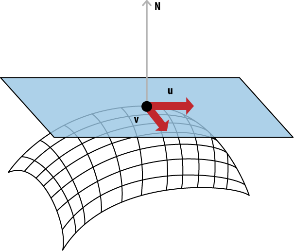
We scoff at mathematicians for living in an artificially ideal world, but we can’t dismiss the math behind normals; we need it to come up with sensible values in the first place. Central to the mathematical notion of a normal is the concept of a tangent plane, depicted in Figure 4-5.

The diagram in Figure 4-5 is, in itself, perhaps the best definition of the tangent plane that I can give you without going into calculus. It’s the plane that “just touches” your surface at a given point P. Think like a mathematician: for them, a plane is minimally defined with three points. So, imagine three points at random positions on your surface, and then create a plane that contains them all. Slowly move the three points toward each other; just before the three points converge, the plane they define is the tangent plane.

The tangent plane can also be defined with tangent and binormal vectors (u and v in Figure 4-5), which are easiest to define within the context of a parametric surface. Each of these correspond to a dimension of the domain; we’ll make use of this when we add normals to our ParametricSurface class.

Finding two vectors in the tangent plane is usually fairly easy. For example, you can take any two sides of a triangle; the two vectors need not be at right angles to each other. Simply take their cross product and unitize the result. For parametric surfaces, the procedure can be summarized with the following pseudocode:

p = Evaluate(s, t)
u = Evaluate(s + ds, t) - p
v = Evaluate(s, t + dt) - p
N = Normalize(u × v)

Figure 4-5. Normal vector with tangent plane

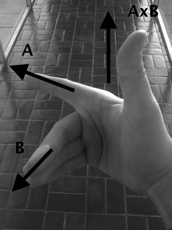
Don’t be frightened by the cross product; I’ll give you a brief refresher. The cross product always generates a vector perpendicular to its two input vectors. You can visualize the cross product of A with B using your right hand. Point your index finger in the direction of A, and then point your middle finger toward B; your thumb now points in the direction of A×B (pronounced “A cross B,” not “A times B”). See Figure 4-6.

Figure 4-6. Righthand rule

Here’s the relevant snippet from our C++ library (see the appendix for a full listing):

template <typename T>
struct Vector3 {
    // ...
    Vector3 Cross(const Vector3& v) const
    {
        return Vector3(y * v.z - z * v.y,
                       z * v.x - x * v.z,
                       x * v.y - y * v.x);
    }
    // ...
    T x, y, z;
};

Normal Transforms Aren’t Normal

Let’s not lose focus of why we’re generating normals in the first place: they’re required for the lighting algorithms that we cover later in this chapter. Recall from Chapter 2 that vertex position can live in different spaces: object space, world space, and so on. Normal vectors can live in these different spaces too; it turns out that lighting in the vertex shader is often performed in eye space. (There are certain conditions in which it can be done in object space, but that’s a discussion for another day.)

So, we need to transform our normals to eye space. Since vertex positions get transformed by the model-view matrix to bring them into eye space, it follows that normal vectors get transformed the same way, right? Wrong! Actually, wrong sometimes. This is one of the trickier concepts in graphics to understand, so bear with me.

Look at the heart shape in Figure 4-7, and consider the surface normal at a point in the upper-left quadrant (depicted with an arrow). The figure on the far left is the original shape, and the middle figure shows what happens after we translate, rotate, and uniformly shrink the heart. The transformation for the normal vector is almost the same as the model’s transformation; the only difference is that it’s a vector and therefore doesn’t require translation. Removing translation from a 4×4 transformation matrix is easy. Simply extract the upper-left 3×3 matrix, and you’re done.

Figure 4-7. Normal transforms

Now take a look at the figure on the far right, which shows what happens when stretching the model along only its x-axis. In this case, if we were to apply the upper 3×3 of the model-view matrix to the normal vector, we’d get an incorrect result; the normal would no longer be perpendicular to the surface. This shows that simply extracting the upper-left 3×3 matrix from the model-view matrix doesn’t always suffice. I won’t bore you with the math, but it can be shown that the correct transform for normal vectors is actually the inverse-transpose of the model-view matrix, which is the result of two operations: first an inverse, then a transpose.

The inverse matrix of M is denoted M^-1; it’s the matrix that results in the identity matrix when multiplied with the original matrix. Inverse matrices are somewhat nontrivial to compute, so again I’ll refrain from boring you with the math. The transpose matrix, on the other hand, is easy to derive; simply swap the rows and columns of the matrix such that M[i][j] becomes M[j][i].

Transposes are denoted M^T, so the proper transform for normal vectors looks like this:

Don’t forget the middle shape in Figure 4-7; it shows that, at least in some cases, the upper 3×3 of the original model-view matrix can be used to transform the normal vector. In this case, the matrix just happens to be equal to its own inverse-transpose; such matrices are called orthogonal. Rigid body transformations like rotation and uniform scale always result in orthogonal matrices.

Why did I bore you with all this mumbo jumbo about inverses and normal transforms? Two reasons. First, in ES 1.1, keeping nonuniform scale out of your matrix helps performance because OpenGL can avoid computing the inverse-transpose of the model-view. Second, for ES 2.0, you need to understand nitty-gritty details like this anyway to write sensible lighting shaders!

Generating Normals from Parametric Surfaces

Enough academic babble; let’s get back to coding. Since our goal here is to add lighting to ModelViewer, we need to implement the generation of normal vectors. Let’s tweak ISurface in Interfaces.hpp by adding a flags parameter to GenerateVertices, as shown in Example 4-7. New or modified lines are shown in bold.

Example 4-7. Modifying ISurface with support for normals

enum VertexFlags {
    VertexFlagsNormals = 1 << 0,
    VertexFlagsTexCoords = 1 << 1,
};

struct ISurface {
    virtual int GetVertexCount() const = 0;
    virtual int GetLineIndexCount() const = 0;
    virtual int GetTriangleIndexCount() const = 0;
    virtual void GenerateVertices(vector<float>& vertices,
                                  unsigned char flags = 0) const = 0;
    virtual void GenerateLineIndices(vector<unsigned short>& indices) const = 0;
    virtual void 
      GenerateTriangleIndices(vector<unsigned short>& indices) const = 0;
    virtual ~ISurface() {}
};

The argument we added to GenerateVertices could have been a boolean instead of a bit mask, but we’ll eventually want to feed additional vertex attributes to OpenGL, such as texture coordinates. For now, just ignore the VertexFlagsTexCoords flag; it’ll come in handy in the next chapter.

Next we need to open ParametricSurface.hpp and make the complementary change to the class declaration of ParametricSurface, as shown in Example 4-8. We’ll also add a new protected method called InvertNormal, which derived classes can optionally override.

Example 4-8. ParametricSurface class declaration

class ParametricSurface : public ISurface {
public:
    int GetVertexCount() const;
    int GetLineIndexCount() const;
    int GetTriangleIndexCount() const;
    void GenerateVertices(vector<float>& vertices, unsigned char flags) const;
    void GenerateLineIndices(vector<unsigned short>& indices) const;
    void GenerateTriangleIndices(vector<unsigned short>& indices) const;
protected:
    void SetInterval(const ParametricInterval& interval);
    virtual vec3 Evaluate(const vec2& domain) const = 0;
    virtual bool InvertNormal(const vec2& domain) const { return false; }
private:
    vec2 ComputeDomain(float i, float j) const;
    vec2 m_upperBound;
    ivec2 m_slices;
    ivec2 m_divisions;
};

Next let’s open ParametericSurface.cpp and replace the implementation of GenerateVertices, as shown in Example 4-9.

Example 4-9. Adding normals to ParametricSurface::GenerateVertices

void ParametricSurface::GenerateVertices(vector<float>& vertices,
                                         unsigned char flags) const
{
    int floatsPerVertex = 3;
    if (flags & VertexFlagsNormals)
        floatsPerVertex += 3;

    vertices.resize(GetVertexCount() * floatsPerVertex);
    float* attribute = (float*) &vertices[0];

    for (int j = 0; j < m_divisions.y; j++) {
        for (int i = 0; i < m_divisions.x; i++) {

            // Compute Position
            vec2 domain = ComputeDomain(i, j);
            vec3 range = Evaluate(domain);
            attribute = range.Write(attribute);

            // Compute Normal
            if (flags & VertexFlagsNormals) {
                float s = i, t = j;

                // Nudge the point if the normal is indeterminate.
                if (i == 0) s += 0.01f;
                if (i == m_divisions.x - 1) s -= 0.01f;
                if (j == 0) t += 0.01f;
                if (j == m_divisions.y - 1) t -= 0.01f;
                
                // Compute the tangents and their cross product.
                vec3 p = Evaluate(ComputeDomain(s, t));
                vec3 u = Evaluate(ComputeDomain(s + 0.01f, t)) - p;
                vec3 v = Evaluate(ComputeDomain(s, t + 0.01f)) - p;
                vec3 normal = u.Cross(v).Normalized();
                if (InvertNormal(domain))
                    normal = -normal;
                attribute = normal.Write(attribute);
            }
        }
    }
}

Compute the position of the vertex by calling Evaluate, which has a unique implementation for each subclass.

Copy the vec3 position into the flat floating-point buffer. The Write method returns an updated pointer.

Surfaces might be nonsmooth in some places where the normal is impossible to determine (for example, at the apex of the cone). So, we have a bit of a hack here, which is to nudge the point of interest in the problem areas.

As covered in Feeding OpenGL with Normals, compute the two tangent vectors, and take their cross product.

Subclasses are allowed to invert the normal if they want. (If the normal points away from the light source, then it’s considered to be the back of the surface and therefore looks dark.) The only shape that overrides this method is the Klein bottle.

Copy the normal vector into the data buffer using its Write method.

This completes the changes to ParametricSurface. You should be able to build ModelViewer at this point, but it will look the same since we have yet to put the normal vectors to good use. That comes next.

Lighting Up

Drawing is deception.

—M. C. Escher

The foundations of real-time graphics are rarely based on principles from physics and optics. In a way, the lighting equations we’ll cover in this section are cheap hacks, simple models based on rather shallow empirical observations. We’ll be demonstrating three different lighting models: ambient lighting (subtle, monotone light), diffuse lighting (the dull matte component of reflection), and specular lighting (the shiny spot on a fresh red apple). Figure 4-8 shows how these three lighting models can be combined to produce a high-quality image.

Figure 4-8. Ambient + diffuse + specular = final

Of course, in the real world, there are no such things as “diffuse photons” and “specular photons.” Don’t be disheartened by this pack of lies! Computer graphics is always just a great big hack at some level, and knowing this will make you stronger. Even the fact that colors are ultimately represented by a red-green-blue triplet has more to do with human perception than with optics. The reason we use RGB? It happens to match the three types of color-sensing cells in the human retina! A good graphics programmer can think like a politician and use lies to his advantage.

Ho-Hum Ambiance

Realistic ambient lighting, with the soft, muted shadows that it conjures up, can be very complex to render (you can see an example of ambient occlusion in Baked Lighting), but ambient lighting in the context of OpenGL usually refers to something far more trivial: a solid, uniform color. Calling this “lighting” is questionable since its intensity is not impacted by the position of the light source or the orientation of the surface, but it is often combined with the other lighting models to produce a brighter surface.

Matte Paint with Diffuse Lighting

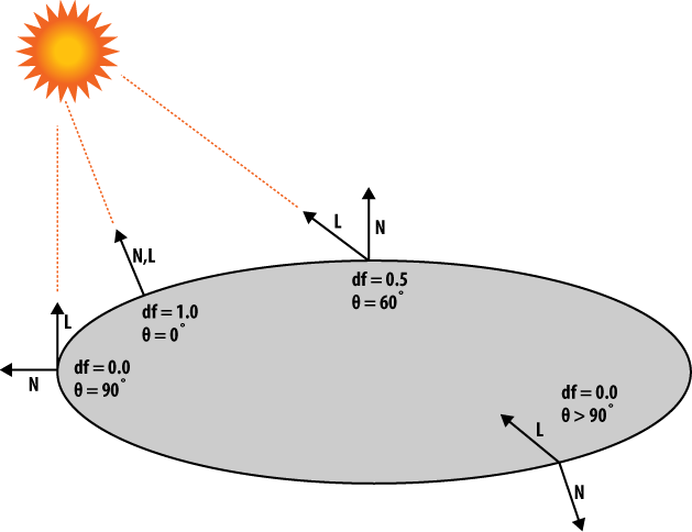
The most common form of real-time lighting is diffuse lighting, which varies its brightness according to the angle between the surface and the light source. Also known as lambertian reflection, this form of lighting is predominant because it’s simple to compute, and it adequately conveys depth to the human eye. Figure 4-9 shows how diffuse lighting works. In the diagram, L is the unit length vector pointing to the light source, and N is the surface normal, which is a unit-length vector that’s perpendicular to the surface. We’ll learn how to compute N later in the chapter.

Figure 4-9. Diffuse lighting

The diffuse factor (known as df in Figure 4-9) lies between 0 and 1 and gets multiplied with the light intensity and material color to produce the final diffuse color, as shown in Equation 4-1.

Equation 4-1. Diffuse color

df is computed by taking the dot product of the surface normal with the light direction vector and then clamping the result to a non-negative number, as shown in Equation 4-2.

Equation 4-2. Diffuse coefficient

The dot product is another operation that you might need a refresher on. When applied to two unit-length vectors (which is what we’re doing for diffuse lighting), you can think of the dot product as a way of measuring the angle between the vectors. If the two vectors are perpendicular to each other, their dot product is zero; if they point away from each other, their dot product is negative. Specifically, the dot product of two unit vectors is the cosine of the angle between them. To see how to compute the dot product, here’s a snippet from our C++ vector library (see the appendix for a complete listing):

template <typename T>
struct Vector3 {
    // ...
    T Dot(const Vector3& v) const
    {
        return x * v.x + y * v.y + z * v.z;
    }
    // ...
    T x, y, z;
};

Warning

Don’t confuse the dot product with the cross product! For one thing, cross products produce vectors, while dot products produce scalars.

With OpenGL ES 1.1, the math required for diffuse lighting is done for you behind the scenes; with 2.0, you have to do the math yourself in a shader. You’ll learn both methods later in the chapter.

The L vector in Equation 4-2 can be computed like this:

In practice, you can often pretend that the light is so far away that all vertices are at the origin. The previous equation then simplifies to the following:

When you apply this optimization, you’re said to be using an infinite light source. Taking each vertex position into account is slower but more accurate; this is a positional light source.

Give It a Shine with Specular

I guess you could say the Overlook Hotel here has somethin’ almost like “shining.”

—Mr. Hallorann to Danny, The Shining

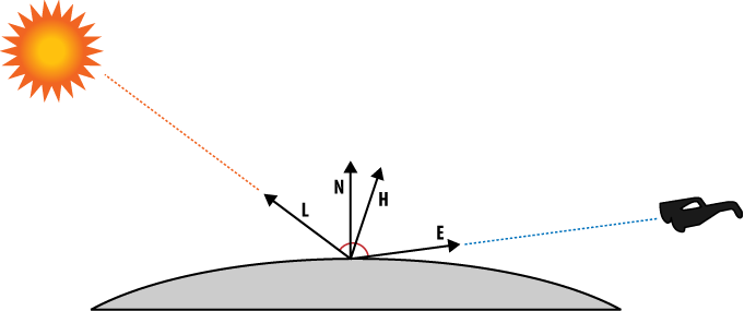
Diffuse lighting is not affected by the position of the camera; the diffuse brightness of a fixed point stays the same, no matter which direction you observe it from. This is in contrast to specular lighting, which moves the area of brightness according to your eye position, as shown in Figure 4-10. Specular lighting mimics the shiny highlight seen on polished surfaces. Hold a shiny apple in front of you, and shift your head to the left and right; you’ll see that the apple’s shiny spot moves with you. Specular is more costly to compute than diffuse because it uses exponentiation to compute falloff. You choose the exponent according to how you want the material to look; the higher the exponent, the shinier the model.

Figure 4-10. Specular lighting

The H vector in Figure 4-10 is called the half-angle because it divides the angle between the light and the camera in half. Much like diffuse lighting, the goal is to compute an intensity coefficient (in this case, sf) between 0 and 1. Equation 4-3 shows how to compute sf.

Equation 4-3. Specular lighting

In practice, you can often pretend that the viewer is infinitely far from the vertex, in which case the E vector is substituted with (0, 0, 1). This technique is called infinite viewer. When E is used, this is called local viewer.

Adding Light to ModelViewer

We’ll first add lighting to the OpenGL ES 1.1 backend since it’s much less involved than the 2.0 variant. Example 4-10 shows the new Initialize method (unchanged portions are replaced with ellipses for brevity).

Example 4-10. ES1::RenderingEngine::Initialize

void RenderingEngine::Initialize(const vector<ISurface*>& surfaces)
{
    vector<ISurface*>::const_iterator surface;
    for (surface = surfaces.begin(); surface != surfaces.end(); ++surface) {
        
        // Create the VBO for the vertices.
        vector<float> vertices;
        (*surface)->GenerateVertices(vertices, VertexFlagsNormals);
        GLuint vertexBuffer;
        glGenBuffers(1, &vertexBuffer);
        glBindBuffer(GL_ARRAY_BUFFER, vertexBuffer);
        glBufferData(GL_ARRAY_BUFFER,
                     vertices.size() * sizeof(vertices[0]),
                     &vertices[0],
                     GL_STATIC_DRAW);
        
        // Create a new VBO for the indices if needed.
        ...
    }

    // Set up various GL state.
    glEnableClientState(GL_VERTEX_ARRAY);
    glEnableClientState(GL_NORMAL_ARRAY);
    glEnable(GL_LIGHTING);
    glEnable(GL_LIGHT0);
    glEnable(GL_DEPTH_TEST);

    // Set up the material properties.
    vec4 specular(0.5f, 0.5f, 0.5f, 1);
    glMaterialfv(GL_FRONT_AND_BACK, GL_SPECULAR, specular.Pointer());
    glMaterialf(GL_FRONT_AND_BACK, GL_SHININESS, 50.0f);

    m_translation = mat4::Translate(0, 0, -7);
}

Tell the ParametricSurface object that we need normals by passing in the new VertexFlagsNormals flag.

Enable two vertex attributes: one for position, the other for surface normal.

Enable lighting, and turn on the first light source (known as GL_LIGHT0). The iPhone supports up to eight light sources, but we’re using only one.

The default specular color is black, so here we set it to gray and set the specular exponent to 50. We’ll set diffuse later.

Example 4-10 uses some new OpenGL functions: glMaterialf and glMaterialfv. These are useful only when lighting is turned on, and they are unique to ES 1.1—with 2.0 you’d use glVertexAttrib instead. The declarations for these functions are the following:

void glMaterialf(GLenum face, GLenum pname, GLfloat param);
void glMaterialfv(GLenum face, GLenum pname, const GLfloat *params);

The face parameter is a bit of a carryover from desktop OpenGL, which allows the back and front sides of a surface to have different material properties. For OpenGL ES, this parameter must always be set to GL_FRONT_AND_BACK.

The pname parameter can be one of the following:

GL_SHININESS

This specifies the specular exponent as a float between 0 and 128. This is the only parameter that you set with glMaterialf; all other parameters require glMaterialfv because they have four floats each.

GL_AMBIENT

This specifies the ambient color of the surface and requires four floats (red, green, blue, alpha). The alpha value is ignored, but I always set it to one just to be safe.

GL_SPECULAR

This specifies the specular color of the surface and also requires four floats, although alpha is ignored.

GL_EMISSION

This specifies the emission color of the surface. We haven’t covered emission because it’s so rarely used. It’s similar to ambient except that it’s unaffected by light sources. This can be useful for debugging; if you want to verify that a surface of interest is visible, set its emission color to white. Like ambient and specular, it requires four floats and alpha is ignored.

GL_DIFFUSE

This specifies the diffuse color of the surface and requires four floats. The final alpha value of the pixel originates from the diffuse color.

GL_AMBIENT_AND_DIFFUSE

Using only one function call, this allows you to specify the same color for both ambient and diffuse.

When lighting is enabled, the final color of the surface is determined at run time, so OpenGL ignores the color attribute that you set with glColor4f or GL_COLOR_ARRAY (see Table 2-2). Since you’d specify the color attribute only when lighting is turned off, it’s often referred to as nonlit color.

Note

As an alternative to calling glMaterialfv, you can embed diffuse and ambient colors into the vertex buffer itself, through a mechanism called color material. When enabled, this redirects the nonlit color attribute into the GL_AMBIENT and GL_DIFFUSE material parameters. You can enable it by calling glEnable(GL_COLOR_MATERIAL).

Next we’ll flesh out the Render method so that it uses normals, as shown in Example 4-11. New/changed lines are in bold. Note that we moved up the call to glMatrixMode; this is explained further in the callouts that follow the listing.

Example 4-11. ES1::RenderingEngine::Render

void RenderingEngine::Render(const vector<Visual>& visuals) const
{
    glClearColor(0.5f, 0.5f, 0.5f, 1);
    glClear(GL_COLOR_BUFFER_BIT | GL_DEPTH_BUFFER_BIT);
    
    vector<Visual>::const_iterator visual = visuals.begin();
    for (int visualIndex = 0; 
         visual != visuals.end(); 
         ++visual, ++visualIndex) 
    {
        
        // Set the viewport transform.
        ivec2 size = visual->ViewportSize;
        ivec2 lowerLeft = visual->LowerLeft;
        glViewport(lowerLeft.x, lowerLeft.y, size.x, size.y);
        
        // Set the light position.
        glMatrixMode(GL_MODELVIEW);
        glLoadIdentity();
        vec4 lightPosition(0.25, 0.25, 1, 0);
        glLightfv(GL_LIGHT0, GL_POSITION, lightPosition.Pointer());
        
        // Set the model-view transform.
        mat4 rotation = visual->Orientation.ToMatrix();
        mat4 modelview = rotation * m_translation;
        glLoadMatrixf(modelview.Pointer());
        
        // Set the projection transform.
        float h = 4.0f * size.y / size.x;
        mat4 projection = mat4::Frustum(-2, 2, -h / 2, h / 2, 5, 10);
        glMatrixMode(GL_PROJECTION);
        glLoadMatrixf(projection.Pointer());
        
        // Set the diffuse color.
        vec3 color = visual->Color * 0.75f;
        vec4 diffuse(color.x, color.y, color.z, 1);
        glMaterialfv(GL_FRONT_AND_BACK, GL_DIFFUSE, diffuse.Pointer());

        // Draw the surface.
        int stride = 2 * sizeof(vec3);
        const Drawable& drawable = m_drawables[visualIndex];
        glBindBuffer(GL_ARRAY_BUFFER, drawable.VertexBuffer);
        glVertexPointer(3, GL_FLOAT, stride, 0);
        const GLvoid* normalOffset = (const GLvoid*) sizeof(vec3);
        glNormalPointer(GL_FLOAT, stride, normalOffset);
        glBindBuffer(GL_ELEMENT_ARRAY_BUFFER, drawable.IndexBuffer);
        glDrawElements(GL_TRIANGLES, drawable.IndexCount, GL_UNSIGNED_SHORT, 0);
    }
}

Set the position of GL_LIGHT0. Be careful about when you make this call, because OpenGL applies the current model-view matrix to the position, much like it does to vertices. Since we don’t want the light to rotate along with the model, here we’ve reset the model-view before setting the light position.

The nonlit version of the app used glColor4f in the section that started with the comment // Set the color. We’re replacing that with glMaterialfv. More on this later.

Point OpenGL to the right place in the VBO for obtaining normals. Position comes first, and it’s a vec3, so the normal offset is sizeof(vec3).

That’s it! Figure 4-11 depicts the app now that lighting has been added. Since we haven’t implemented the ES 2.0 renderer yet, you’ll need to enable the ForceES1 constant at the top of GLView.mm.

Figure 4-11. ModelViewer with lighting

Using Light Properties

Example 4-11 introduced a new OpenGL function for modifying light parameters, glLightfv:

void glLightfv(GLenum light, GLenum pname, const GLfloat *params);

The light parameter identifies the light source. Although we’re using only one light source in ModelViewer, up to eight are allowed (GL_LIGHT0–GL_LIGHT7).

The pname argument specifies the light property to modify. OpenGL ES 1.1 supports 10 light properties:

GL_AMBIENT, GL_DIFFUSE, GL_SPECULAR

As you’d expect, each of these takes four floats to specify a color. Note that light colors alone do not determine the hue of the surface; they get multiplied with the surface colors specified by glMaterialfv.

GL_POSITION

The position of the light is specified with four floats. If you don’t set the light’s position, it defaults to (0, 0, 1, 0). The W component should be 0 or 1, where 0 indicates an infinitely distant light. Such light sources are just as bright as normal light sources, but their “rays” are parallel. This is computationally cheaper because OpenGL does not bother recomputing the L vector (see Figure 4-9) at every vertex.

GL_SPOT_DIRECTION, GL_SPOT_EXPONENT, GL_SPOT_CUTOFF

You can restrict a light’s area of influence to a cone using these parameters. Don’t set these parameters if you don’t need them; doing so can degrade performance. I won’t go into detail about spotlights since they are somewhat esoteric to ES 1.1, and you can easily write a shader in ES 2.0 to achieve a similar effect. Consult an OpenGL reference to see how to use spotlights (see the section Further Reading).

GL_CONSTANT_ATTENUATION, GL_LINEAR_ATTENUATION, GL_QUADRATIC_ATTENUATION

These parameters allow you to dim the light intensity according to its distance from the object. Much like spotlights, attenuation is surely covered in your favorite OpenGL reference book. Again, be aware that setting these parameters could impact your frame rate.

You may’ve noticed that the inside of the cone appears especially dark. This is because the normal vector is facing away from the light source. On third-generation iPhones and iPod touches, you can enable a feature called two-sided lighting, which inverts the normals on back-facing triangles, allowing them to be lit. It’s enabled like this:

glLightModelf(GL_LIGHT_MODEL_TWO_SIDE, GL_TRUE);

Use this function with caution, because it is not supported on older iPhones. One way to avoid two-sided lighting is to redraw the geometry at a slight offset using flipped normals. This effectively makes your one-sided surface into a two-sided surface. For example, in the case of our cone shape, we could draw another equally sized cone that’s just barely “inside” the original cone.

Note

Just like every other lighting function, glLightModelf doesn’t exist under ES 2.0. With ES 2.0, you can achieve two-sided lighting by using a special shader variable called gl_FrontFacing.

Shaders Demystified

Before we add lighting to the ES 2.0 rendering engine of ModelViewer, let’s go over some shader fundamentals. What exactly is a shader? In Chapter 1, we mentioned that shaders are relatively small snippets of code that run on the graphics processor and that thousands of shader instances can execute simultaneously.

Let’s dissect the simple vertex shader that we’ve been using in our sample code so far, repeated here in Example 4-12.

Example 4-12. Simple.vert

attribute vec4 Position; 
attribute vec4 SourceColor; 
varying vec4 DestinationColor; 
uniform mat4 Projection; 
uniform mat4 Modelview; 

void main(void) 
{
    DestinationColor = SourceColor; 
    gl_Position = Projection * Modelview * Position; 
}

Declare two 4D floating-point vectors with the attribute storage qualifier. Vertex shaders have read-only access to attributes.

Declare a 4D floating-point vector as a varying. The vertex shader must write to all varyings that it declares—if it doesn’t, OpenGL’s shader compiler will report an error. The initial value is undefined.

Declare two 4×4 matrices as uniforms. Much like attributes, the vertex shader has read-only access to uniforms. But unlike vertex attributes, uniforms cannot change from one vertex to the next.

The entry point to the shader. Some shading languages let you define your own entry point, but with GLSL, it’s always main.

No lighting or fancy math here; just pass the SourceColor attribute into the DestinationColor varying.

Here we transform the position by the projection and model-view matrices, much like OpenGL ES 1.1 automatically does on our behalf. Note the usage of gl_Position, which is a special output variable built into the vertex shading language.

The keywords attribute, uniform, and varying are storage qualifiers in GLSL. Table 4-1 summarizes the five storage qualifiers available in GLSL.

Table 4-1. GLSL storage qualifiers

Qualifier	Maximum permitted[a]	Readable from VS	Writable from VS	Readable from FS	Writable from FS
default	N/A	Yes	Yes	Yes	Yes
const	N/A	Yes	Yes	Yes	Yes
attribute	8 vec4	Yes	No	No	No
uniform	512 scalars (VS), 64 scalars (FS)	Yes	No	Yes	No
varying	8 vec4	No	Yes	Yes	No
[a] Implementation-specific data; pertains only to the iPhone 3GS.

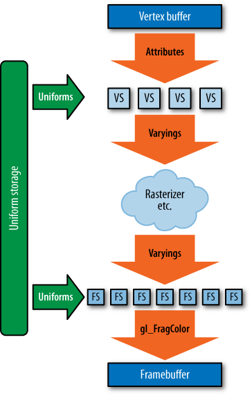
Figure 4-12 shows one way to visualize the flow of shader data. Be aware that this diagram is very simplified; for example, it does not include blocks for texture memory or program storage.

Figure 4-12. Shader-centric view of OpenGL (VS = vertex shader, FS = fragment shader)

The fragment shader we’ve been using so far is incredibly boring, as shown in Example 4-13.

Example 4-13. Boring fragment shader

varying lowp vec4 DestinationColor;

void main(void)
{
    gl_FragColor = DestinationColor;
}

This declares a 4D floating-point varying (read-only) with lowp precision. Precision qualifiers are required for floating-point types in fragment shaders.

The entry point to every fragment shader is its main function.

gl_FragColor is a special built-in vec4 that indicates the output of the fragment shader.

Perhaps the most interesting new concept here is the precision qualifier. Fragment shaders require a precision qualifier for all floating-point declarations. The valid qualifiers are lowp, mediump, and highp. The GLSL specification gives implementations some leeway in the underlying binary format that corresponds to each of these qualifiers; Table 4-2 shows specific details for the graphics processor in the iPhone 3GS.

Note

An alternative to specifying precision in front of every type is to supply a default using the precision keyword. Vertex shaders implicitly have a default floating-point precision of highp. To create a similar default in your fragment shader, add precision highp float; to the top of your shader.

Table 4-2. Floating-point precision in third-generation devices

Qualifier	Underlying type	Range	Typical usage
highp	32-bit floating point	[−9.999999×1096,+9.999999×1096]	colors, normals
mediump	16-bit floating point	[–65520, +65520]	texture coordinates
lowp	10-bit fixed point	[–2, +2]	vertex positions, matrices

Also of interest in Example 4-13 is the gl_FragColor variable, which is a bit of a special case. It’s a variable that is built into the language itself and always refers to the color that gets applied to the framebuffer. The fragment shading language also defines the following built-in variables:

gl_FragData[0]

gl_FragData is an array of output colors that has only one element. This exists in OpenGL ES only for compatibility reasons; use gl_FragColor instead.

gl_FragCoord

This is an input variable that contains window coordinates for the current fragment, which is useful for image processing.

gl_FrontFacing

Use this boolean input variable to implement two-sided lighting. Front faces are true; back faces are false.

gl_PointCoord

This is an input texture coordinate that’s used only for point sprite rendering; we’ll cover it in the section Rendering Confetti, Fireworks, and More: Point Sprites.

Adding Shaders to ModelViewer

OpenGL ES 2.0 does not automatically perform lighting math behind the scenes; instead, it relies on developers to provide it with shaders that perform whatever type of lighting they desire. Let’s come up with a vertex shader that mimics the math done by ES 1.1 when lighting is enabled.

To keep things simple, we’ll use the infinite light source model for diffuse (Feeding OpenGL with Normals) combined with the infinite viewer model for specular (Give It a Shine with Specular). We’ll also assume that the light is white. Example 4-14 shows the pseudocode.

Example 4-14. Basic lighting pseudocode

vec3 ComputeLighting(vec3 normal)
{
    N = NormalMatrix * normal
    L = Normalize(LightPosition)
    E = (0, 0, 1)
    H = Normalize(L + E)
    df = max(0, N ∙ L)
    sf = max(0, N ∙ H)
    sf = sf ^ Shininess
    return AmbientMaterial + DiffuseMaterial * df + SpecularMaterial * sf
}

Note the NormalMatrix variable in the pseudocode; it would be silly to recompute the inverse-transpose of the model-view at every vertex, so we’ll compute it up front in the application code then pass it in as the NormalMatrix uniform. In many cases, it happens to be equivalent to the model-view, but we’ll leave it to the application to decide how to compute it.

Let’s add a new file to the ModelViewer project called SimpleLighting.vert for the lighting algorithm. In Xcode, right-click the Shaders folder, and choose Add→New file. Select the Empty File template in the Other category. Name it SimpleLighting.vert, and add /Shaders after the project folder name in the location field. Deselect the checkbox in the Targets list, and click Finish.

Example 4-15 translates the pseudocode into GLSL. To make the shader usable in a variety of situations, we use uniforms to store light position, specular, and ambient properties. A vertex attribute is used to store the diffuse color; for many models, the diffuse color may vary on a per-vertex basis (although in our case it does not). This would allow us to use a single draw call to draw a multicolored model.

Warning

Remember, we’re leaving out the STRINGIFY macros in all shader listings from here on out, so take a look at Example 1-13 to see how to add that macro to this file.

Example 4-15. SimpleLighting.vert

attribute vec4 Position;
attribute vec3 Normal;
attribute vec3 DiffuseMaterial;

uniform mat4 Projection;
uniform mat4 Modelview;
uniform mat3 NormalMatrix;
uniform vec3 LightPosition;
uniform vec3 AmbientMaterial;
uniform vec3 SpecularMaterial;
uniform float Shininess;

varying vec4 DestinationColor;

void main(void)
{
    vec3 N = NormalMatrix * Normal;
    vec3 L = normalize(LightPosition);
    vec3 E = vec3(0, 0, 1);
    vec3 H = normalize(L + E);

    float df = max(0.0, dot(N, L));
    float sf = max(0.0, dot(N, H));
    sf = pow(sf, Shininess);

    vec3 color = AmbientMaterial + df * DiffuseMaterial + sf * SpecularMaterial;
    
    DestinationColor = vec4(color, 1);
    gl_Position = Projection * Modelview * Position;
}

Take a look at the pseudocode in Example 4-14; the vertex shader is an implementation of that. The main difference is that GLSL requires you to qualify many of the variables as being attributes, uniforms, or varyings. Also note that in its final code line, Example 4-15 performs the standard transformation of the vertex position, just as it did for the nonlit case.

Warning

GLSL is a bit different from many other languages in that it does not autopromote literals from integers to floats. For example, max(0, myFloat) generates a compile error, but max(0.0, myFloat) does not. On the other hand, constructors for vector-based types do perform conversion implicitly; it’s perfectly legal to write either vec2(0, 0) or vec3(0.0, 0.0).

New Rendering Engine

To create the ES 2.0 backend to ModelViewer, let’s start with the ES 1.1 variant and make the following changes, some of which should be familiar by now:

1. Copy the contents of RenderingEngine.ES1.cpp into RenderingEngine.ES2.cpp.

2. Remove the _OES and OES suffixes from the FBO code.

3. Change the namespace from ES1 to ES2.

4. Change the two #includes to point to the ES2 folder rather than the ES1 folder.

5. Add the BuildShader and BuildProgram methods (see Example 1-18). You must change all instances of RenderingEngine2 to RenderingEngine because we are using namespaces to distinguish between the 1.1 and 2.0 renderers.

6. Add declarations for BuildShader and BuildProgram to the class declaration as shown in Example 1-15.

7. Add the #include for iostream as shown in Example 1-15.

Now that the busywork is out of the way, let’s add declarations for the uniform handles and attribute handles that are used to communicate with the vertex shader. Since the vertex shader is now much more complex than the simple pass-through program we’ve been using, let’s group the handles into simple substructures, as shown in Example 4-16. Add this code to RenderingEngine.ES2.cpp, within the namespace declaration, not above it. (The bold part of the listing shows the two lines you must add to the class declaration’s private: section.)

Example 4-16. ES2::RenderingEngine structures

#define STRINGIFY(A)  #A
#include "../Shaders/SimpleLighting.vert"
#include "../Shaders/Simple.frag"

struct UniformHandles {
    GLuint Modelview;
    GLuint Projection;
    GLuint NormalMatrix;
    GLuint LightPosition;
};
    
struct AttributeHandles {
    GLint Position;
    GLint Normal;
    GLint Ambient;
    GLint Diffuse;
    GLint Specular;
    GLint Shininess;
};

class RenderingEngine : public IRenderingEngine {
    // ...
    UniformHandles m_uniforms;
    AttributeHandles m_attributes;
};

Next we need to change the Initialize method so that it compiles the shaders, extracts the handles to all the uniforms and attributes, and sets up some default material colors. Replace everything from the comment // Set up various GL state to the end of the method with the contents of Example 4-17.

Example 4-17. ES2::RenderingEngine::Initialize()

...

// Create the GLSL program.
GLuint program = BuildProgram(SimpleVertexShader, SimpleFragmentShader);
glUseProgram(program);

// Extract the handles to attributes and uniforms.
m_attributes.Position = glGetAttribLocation(program, "Position");
m_attributes.Normal = glGetAttribLocation(program, "Normal");
m_attributes.Ambient = glGetAttribLocation(program, "AmbientMaterial");
m_attributes.Diffuse = glGetAttribLocation(program, "DiffuseMaterial");
m_attributes.Specular = glGetAttribLocation(program, "SpecularMaterial");
m_attributes.Shininess = glGetAttribLocation(program, "Shininess"); 
m_uniforms.Projection = glGetUniformLocation(program, "Projection");
m_uniforms.Modelview = glGetUniformLocation(program, "Modelview");
m_uniforms.NormalMatrix = glGetUniformLocation(program, "NormalMatrix");
m_uniforms.LightPosition = glGetUniformLocation(program, "LightPosition");

// Set up some default material parameters.
glVertexAttrib3f(m_attributes.Ambient, 0.04f, 0.04f, 0.04f);
glVertexAttrib3f(m_attributes.Specular, 0.5, 0.5, 0.5);
glVertexAttrib1f(m_attributes.Shininess, 50);

// Initialize various state.
glEnableVertexAttribArray(m_attributes.Position);
glEnableVertexAttribArray(m_attributes.Normal);
glEnable(GL_DEPTH_TEST);

// Set up transforms.
m_translation = mat4::Translate(0, 0, -7);

Next let’s replace the Render() method, shown in Example 4-18.

Example 4-18. ES2::RenderingEngine::Render()

void RenderingEngine::Render(const vector<Visual>& visuals) const
{
    glClearColor(0, 0.125f, 0.25f, 1);
    glClear(GL_COLOR_BUFFER_BIT | GL_DEPTH_BUFFER_BIT);

    vector<Visual>::const_iterator visual = visuals.begin();
    for (int visualIndex = 0; 
         visual != visuals.end(); 
         ++visual, ++visualIndex) {

        // Set the viewport transform.
        ivec2 size = visual->ViewportSize;
        ivec2 lowerLeft = visual->LowerLeft;
        glViewport(lowerLeft.x, lowerLeft.y, size.x, size.y);
        
        // Set the light position.
        vec4 lightPosition(0.25, 0.25, 1, 0);
        glUniform3fv(m_uniforms.LightPosition, 1, lightPosition.Pointer());

        // Set the model-view transform.
        mat4 rotation = visual->Orientation.ToMatrix();
        mat4 modelview = rotation * m_translation;
        glUniformMatrix4fv(m_uniforms.Modelview, 1, 0, modelview.Pointer());
        
        // Set the normal matrix.
        // It's orthogonal, so its Inverse-Transpose is itself!
        mat3 normalMatrix = modelview.ToMat3();
        glUniformMatrix3fv(m_uniforms.NormalMatrix, 1, 
                           0, normalMatrix.Pointer());

        // Set the projection transform.
        float h = 4.0f * size.y / size.x;
        mat4 projectionMatrix = mat4::Frustum(-2, 2, -h / 2, h / 2, 5, 10);
        glUniformMatrix4fv(m_uniforms.Projection, 1, 
                           0, projectionMatrix.Pointer());
        
        // Set the diffuse color.
        vec3 color = visual->Color * 0.75f;
        glVertexAttrib4f(m_attributes.Diffuse, color.x, 
                         color.y, color.z, 1);
        
        // Draw the surface.
        int stride = 2 * sizeof(vec3);
        const GLvoid* offset = (const GLvoid*) sizeof(vec3);
        GLint position = m_attributes.Position;
        GLint normal = m_attributes.Normal;
        const Drawable& drawable = m_drawables[visualIndex];
        glBindBuffer(GL_ARRAY_BUFFER, drawable.VertexBuffer);
        glVertexAttribPointer(position, 3, GL_FLOAT, 
                              GL_FALSE, stride, 0);
        glVertexAttribPointer(normal, 3, GL_FLOAT, GL_FALSE, 
                              stride, offset);
        glBindBuffer(GL_ELEMENT_ARRAY_BUFFER, drawable.IndexBuffer);
        glDrawElements(GL_TRIANGLES, drawable.IndexCount, 
                       GL_UNSIGNED_SHORT, 0);
    }
}

That’s it for the ES 2.0 backend! Turn off the ForceES1 switch in GLView.mm, and you should see something very similar to the ES 1.1 screenshot shown in Figure 4-11.

Per-Pixel Lighting

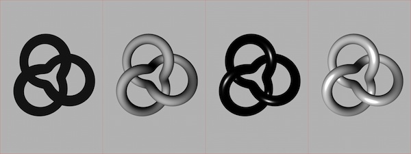
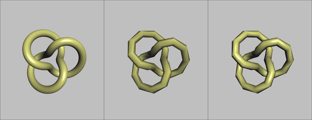
When a model has coarse tessellation, performing the lighting calculations at the vertex level can result in the loss of specular highlights and other detail, as shown in Figure 4-13.

Figure 4-13. Tessellation and lighting (from left to right: infinite tessellation, vertex lighting, and pixel lighting)

One technique to counteract this unattractive effect is per-pixel lighting; this is when most (or all) of the lighting algorithm takes place in the fragment shader.

Warning

Shifting work from the vertex shader to the pixel shader can often be detrimental to performance. I encourage you to experiment with performance before you commit to a specific technique.

The vertex shader becomes vastly simplified, as shown in Example 4-19. It simply passes the diffuse color and eye-space normal to the fragment shader.

Example 4-19. PixelLighting.vert

attribute vec4 Position;
attribute vec3 Normal;
attribute vec3 DiffuseMaterial;

uniform mat4 Projection;
uniform mat4 Modelview;
uniform mat3 NormalMatrix;

varying vec3 EyespaceNormal;
varying vec3 Diffuse;

void main(void)
{
    EyespaceNormal = NormalMatrix * Normal;
    Diffuse = DiffuseMaterial;
    gl_Position = Projection * Modelview * Position;
}

The fragment shader now performs the burden of the lighting math, as shown in Example 4-20. The main distinction it has from its per-vertex counterpart (Example 4-15) is the presence of precision specifiers throughout. We’re using lowp for colors, mediump for the varying normal, and highp for the internal math.

Example 4-20. PixelLighting.frag

varying mediump vec3 EyespaceNormal;
varying lowp vec3 Diffuse;

uniform highp vec3 LightPosition;
uniform highp vec3 AmbientMaterial;
uniform highp vec3 SpecularMaterial;
uniform highp float Shininess;

void main(void)
{
    highp vec3 N = normalize(EyespaceNormal);
    highp vec3 L = normalize(LightPosition);
    highp vec3 E = vec3(0, 0, 1);
    highp vec3 H = normalize(L + E);
    
    highp float df = max(0.0, dot(N, L));
    highp float sf = max(0.0, dot(N, H));
    sf = pow(sf, Shininess);

    lowp vec3 color = AmbientMaterial + df * Diffuse + sf * SpecularMaterial;

    gl_FragColor = vec4(color, 1);
}

Note

To try these, you can replace the contents of your existing .vert and .frag files. Just be sure not to delete the first line with STRINGIFY or the last line with the closing parenthesis and semicolon.

Shifting work from the vertex shader to the fragment shader was simple enough, but watch out: we’re dealing with the normal vector in a sloppy way. OpenGL performs linear interpolation on each component of each varying. This causes inaccurate results, as you might recall from the coverage of quaternions in Chapter 3. Pragmatically speaking, simply renormalizing the incoming vector is often good enough. We’ll cover a more rigorous way of dealing with normals when we present bump mapping in Bump Mapping and DOT3 Lighting.

Toon Shading

Mimicking the built-in lighting functionality in ES 1.1 gave us a fairly painless segue to the world of GLSL. We could continue mimicking more and more ES 1.1 features, but that would get tiresome. After all, we’re upgrading to ES 2.0 to enable new effects, right? Let’s leverage shaders to create a simple effect that would otherwise be difficult (if not impossible) to achieve with ES 1.1.

Toon shading (sometimes cel shading) achieves a cartoony effect by limiting gradients to two or three distinct colors, as shown in Figure 4-14.

Figure 4-14. Toon shading

Assuming you’re already using per-pixel lighting, achieving this is actually incredibly simple; just add the bold lines in Example 4-21.

Example 4-21. ToonShading.frag

varying mediump vec3 EyespaceNormal;
varying lowp vec3 Diffuse;

uniform highp vec3 LightPosition;
uniform highp vec3 AmbientMaterial;
uniform highp vec3 SpecularMaterial;
uniform highp float Shininess;

void main(void)
{
    highp vec3 N = normalize(EyespaceNormal);
    highp vec3 L = normalize(LightPosition);
    highp vec3 E = vec3(0, 0, 1);
    highp vec3 H = normalize(L + E);
    
    highp float df = max(0.0, dot(N, L));
    highp float sf = max(0.0, dot(N, H));
    sf = pow(sf, Shininess);

    if (df < 0.1) df = 0.0;
    else if (df < 0.3) df = 0.3;
    else if (df < 0.6) df = 0.6;
    else df = 1.0;
    
    sf = step(0.5, sf);

    lowp vec3 color = AmbientMaterial + df * Diffuse + sf * SpecularMaterial;

    gl_FragColor = vec4(color, 1);
}

Better Wireframes Using Polygon Offset

The toon shading example belongs to a class of effects called nonphotorealistic effects, often known as NPR effects. Having dangled the carrot of shaders in front of you, I’d now like to show that ES 1.1 can also render some cool effects.

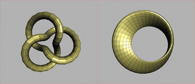
For example, you might want to produce a intentionally faceted look to better illustrate the geometry; this is useful in applications such as CAD visualization or technical illustration. Figure 4-15 shows a two-pass technique whereby the model is first rendered with triangles and then with lines. The result is less messy than the wireframe viewer because hidden lines have been eliminated.

Figure 4-15. Two-pass wireframe with the Trefoil knot and Möbius strip

An issue with this two-pass technique is Z-fighting (see Beware the Scourge of Depth Artifacts). An obvious workaround is translating the first pass backward ever so slightly, or translating the second pass forward. Unfortunately, that approach causes issues because of the nonlinearity of depth precision; some portions of your model would look fine, but other parts may have lines on the opposite side that poke through.

It turns out that both versions of OpenGL ES offer a solution to this specific issue, and it’s called polygon offset. Polygon offset tweaks the Z value of each pixel according to the depth slope of the triangle that it’s in. You can enable and set it up like so:

glEnable(GL_POLYGON_OFFSET_FILL);
glPolygonOffset(factor, units);

factor scales the depth slope, and units gets added to the result. When polygon offset is enabled, the Z values in each triangle get tweaked as follows:

You can find the code to implement this effect in ModelViewer in the downloadable examples (see How to Contact Us). Note that your RenderingEngine class will need to store two VBO handles for index buffers: one for the line indices, the other for the triangle indices. In practice, finding the right values for factor and units almost always requires experimentation.

Warning

Because of a hardware limitation, first- and second-generation iPhones ignore the factor argument in glPolygonOffset.

Flat Shading

One rather obscure feature found only in OpenGL ES 1.1 is flat shading, whereby OpenGL forces the color of each triangle to be uniform. OpenGL performs flat shading by choosing a specific vertex in each triangle and then spreading its associated color throughout the triangle. You can turn it on and off as follows:

glShadeModel(GL_FLAT);   // Turn on flat shading
glShadeModel(GL_SMOOTH); // Turn off flat shading (the default)

I suspect this feature is a bit of a leftover from olden times, when flat shading was a desirable option to increase performance. Nowadays it’s probably useful only for nonphotorealistic rendering. Another way to achieve something similar is simply duplicating the same normal vector at each of the three corners in each triangle; this is one approach you could take for ES 2.0.

Loading Geometry from OBJ Files

So far we’ve been dealing exclusively with a gallery of parametric surfaces. They make a great teaching tool, but parametric surfaces probably aren’t what you’ll be rendering in your app. More likely, you’ll have 3D assets coming from artists who use modeling software such as Maya or Blender.

The first thing to decide on is the file format we’ll use for storing geometry. The COLLADA format was devised to solve the problem of interchange between various 3D packages, but COLLADA is quite complex; it’s capable of conveying much more than just geometry, including effects, physics, and animation.

A more suitable format for our modest purposes is the simple OBJ format, first developed by Wavefront Technologies in the 1980s and still in use today. We won’t go into its full specification here (there are plenty of relevant sources on the Web), but we’ll cover how to load a conformant file that uses a subset of OBJ features.

Warning

Even though the OBJ format is simple and portable, I don’t recommend using it in a production game or application. The parsing overhead can be avoided by inventing your own raw binary format, slurping up the entire file in a single I/O call, and then directly uploading its contents into a vertex buffer. This type of blitz loading can greatly improve the start-up time of your iPhone app.

Note

Another popular geometry file format for the iPhone is PowerVR’s POD format. The PowerVR Insider SDK (discussed in Chapter 5) includes tools and code samples for generating and reading POD files.

Without further ado, Example 4-22 shows an example OBJ file.

Example 4-22. Insanely simple OBJ file

# This is a comment.

v 0.0 1.0 1.0
v 0.0 -1.0 1.0
v 0.0 -1.0 -1.0
v -1.0 1.0 1.0

f 1 2 3
f 2 3 4

Lines that start with a v specify a vertex position using three floats separated by spaces. Lines that start with f specify a “face” with a list of indices into the vertex list. If the OBJ consists of triangles only, then every face has exactly three indices, which makes it a breeze to render with OpenGL. Watch out, though: in OBJ files, indices are one-based, not zero-based as they are in OpenGL.

OBJ also supports vertex normals with lines that start with vn. For a face to refer to a vertex normal, it references it using an index that’s separate from the vertex index, as shown in Example 4-23. The slashes are doubled because the format is actually f v/vt/vn; this example doesn’t use texture coordinates (vt), so it’s blank.

Example 4-23. An OBJ file with vertex normals

v 0.0 1.0 1.0
v 0.0 -1.0 1.0
v 0.0 -1.0 -1.0
vn 1 0 0
f 1//1 2//1 3//1

One thing that’s a bit awkward about this (from an OpenGL standpoint) is that each face specifies separate position indices and normal indices. In OpenGL ES, you only specify a single list of indices; each index simultaneously refers to both a normal and a position.

Because of this complication, the normals found in OBJ files are often ignored in many tools. It’s fairly easy to compute the normals yourself analytically, which we’ll demonstrate soon.

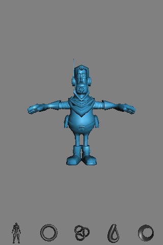
3D artist Christopher Desse has graciously donated some models to the public domain, two of which we’ll be using in ModelViewer: a character named MicroNapalm (the selected model in Figure 4-16) and a ninja character (far left in the tab bar). This greatly enhances the cool factor when you want to show off to your 4-year-old; why have cones and spheres when you can have ninjas?

Figure 4-16. ModelViewer with two OBJ models

Note

I should also mention that I processed Christopher’s OBJ files so that they contain only v lines and f lines with three indices each and that I scaled the models to fit inside a unit cube.

Managing Resource Files

Note that we’ll be loading resources from external files for the first time. Adding file resources to a project is easy in Xcode. Download the two files (micronapalmv2.obj and Ninja.obj) from the examples site, and put them on your desktop or in your Downloads folder.

Create a new folder called Models by right-clicking the ModelViewer root in the Overview pane, and choose Add→New Group. Right-click the new folder, and choose Add→Existing Files. Select the two OBJ files (available from this book’s website) by holding the Command key, and then click Add. In the next dialog box, check the box labeled “Copy items...”, accept the defaults, and then click Add. Done!

The iPhone differs from other platforms in how it handles bundled resources, so it makes sense to create a new interface to shield this from the application engine. Let’s call it IResourceManager, shown in Example 4-24. For now it has a single method that simply returns the absolute path to the folder that has resource files. This may seem too simple to merit its own interface at the moment, but we’ll extend it in future chapters to handle more complex tasks, such as loading image files. Add these lines, and make the change shown in bold to Interface.hpp.

Example 4-24. Adding IResourceManager to Interface.hpp

#include <string>
using std::string;

// ...
struct IResourceManager {
    virtual string GetResourcePath() const = 0;
    virtual ~IResourceManager() {}
};

IResourceManager* CreateResourceManager();

IApplicationEngine* CreateApplicationEngine(IRenderingEngine* renderingEngine,
                                            IResourceManager* resourceManager);

// ...

We added a new argument to CreateApplicationEngine to allow the platform-specific layer to pass in its implementation class. In our case the implementation class needs to be a mixture of C++ and Objective-C. Add a new C++ file to your Xcode project called ResourceManager.mm (don’t create the corresponding .h file), shown in Example 4-25.

Example 4-25. ResourceManager implementation

#import <UIKit/UIKit.h>
#import <QuartzCore/QuartzCore.h>
#import <string>
#import <iostream>
#import "Interfaces.hpp"

using namespace std;

class ResourceManager : public IResourceManager {
public:
    string GetResourcePath() const
    {
        NSString* bundlePath = [[NSBundle mainBundle] resourcePath];
        return [bundlePath UTF8String];
    }
};

IResourceManager* CreateResourceManager()
{
    return new ResourceManager();
}

Retrieve the global mainBundle object, and call its resourcePath method, which returns something like this when running on a simulator:

/Users/username/Library/Application Support/iPhone Simulator
/User/Applications/uuid/ModelViewer.app

When running on a physical device, it returns something like this:

/var/mobile/Applications/uuid/ModelViewer.app

Convert the Objective-C string object into a C++ STL string object using the UTF8String method.

The resource manager should be instanced within the GLView class and passed to the application engine. GLView.h has a field called m_resourceManager, which gets instanced somewhere in initWithFrame and gets passed to CreateApplicationEngine. (This is similar to how we’re already handling the rendering engine.) So, you’ll need to do the following:

1. In GLView.h, add the line IResourceManager* m_resourceManager; to the @private section.

2. In GLView.mm, add the line m_resourceManager = CreateResourceManager(); to initWithFrame (you can add it just above the line if (api == kEAGLRenderingAPIOpenGLES1). Next, add m_resourceManager as the second argument to CreateApplicationEngine.

Next we need to make a few small changes to the application engine per Example 4-26. The lines in bold show how we’re reusing the ISurface interface to avoid changing any code in the rendering engine. Modified/new lines in ApplicationEngine.cpp are shown in bold (make sure you replace the existing assignments to surfaces[0] and surfaces[0] in Initialize):

Example 4-26. Consuming IResourceManager from ApplicationEngine

#include "Interfaces.hpp"
#include "ObjSurface.hpp"

...

class ApplicationEngine : public IApplicationEngine {
public:
    ApplicationEngine(IRenderingEngine* renderingEngine, 
                      IResourceManager* resourceManager);
    ...
private:
    ...
    IResourceManager* m_resourceManager;
};
    
IApplicationEngine* CreateApplicationEngine(IRenderingEngine* renderingEngine, 
                                            IResourceManager* resourceManager)
{
    return new ApplicationEngine(renderingEngine, resourceManager);
}

ApplicationEngine::ApplicationEngine(IRenderingEngine* renderingEngine,
                                     IResourceManager* resourceManager) :
    m_spinning(false),
    m_pressedButton(-1),
    m_renderingEngine(renderingEngine),
    m_resourceManager(resourceManager)
{
...
}

void ApplicationEngine::Initialize(int width, int height)
{
    ...

    string path = m_resourceManager->GetResourcePath();
    surfaces[0] = new ObjSurface(path + "/micronapalmv2.obj");
    surfaces[1] = new ObjSurface(path + "/Ninja.obj");
    surfaces[2] = new Torus(1.4, 0.3);
    surfaces[3] = new TrefoilKnot(1.8f);
    surfaces[4] = new KleinBottle(0.2f);
    surfaces[5] = new MobiusStrip(1);

    ...
}

Implementing ISurface

The next step is creating the ObjSurface class, which implements all the ISurface methods and is responsible for parsing the OBJ file. This class will be more than just a dumb loader; recall that we want to compute surface normals analytically. Doing so allows us to reduce the size of the app, but at the cost of a slightly longer startup time.

We’ll compute the vertex normals by first finding the facet normal of every face and then averaging together the normals from adjoining faces. The C++ implementation of this algorithm is fairly rote, and you can get it from the book’s companion website (http://oreilly.com/catalog/9780596804831); for brevity’s sake, Example 4-27 shows the pseudocode.

Example 4-27. Pseudocode to compute vertex normals from facets

ivec3 faces[faceCount] = read from OBJ
vec3 positions[vertexCount] = read from OBJ
vec3 normals[vertexCount] = { (0,0,0), (0,0,0), ... }

for each face in faces:
    vec3 a = positions[face.Vertex0]
    vec3 b = positions[face.Vertex1]
    vec3 c = positions[face.Vertex2]
    vec3 facetNormal = (a - b) × (c - b)


    normals[face.Vertex0] += facetNormal
    normals[face.Vertex1] += facetNormal
    normals[face.Vertex2] += facetNormal

for each normal in normals:
    normal = normalize(normal)

The mechanics of loading face indices and vertex positions from the OBJ file are somewhat tedious, so you should download ObjSurface.cpp and ObjSurface.hpp from this book’s website (see How to Contact Us) and add them to your Xcode project. Example 4-28 shows the ObjSurface constructor, which loads the vertex indices using the fstream facility in C++. Note that I subtracted one from all vertex indices; watch out for the one-based pitfall!

Example 4-28. ObjSurface constructor

ObjSurface::ObjSurface(const string& name) :
    m_name(name),
    m_faceCount(0),
    m_vertexCount(0)
{
    m_faces.resize(this->GetTriangleIndexCount() / 3);
    ifstream objFile(m_name.c_str());
    vector<ivec3>::iterator face = m_faces.begin();
    while (objFile) {
        char c = objFile.get();
        if (c == 'f') {
            assert(face != m_faces.end() && "parse error");
            objFile >> face->x >> face->y >> face->z;
            *face++ -= ivec3(1, 1, 1);
        }
        objFile.ignore(MaxLineSize, '\n');
    }
    assert(face == m_faces.end() && "parse error");
}

Wrapping Up

We covered quite a bit of territory in this chapter: we took a deep dive into GLSL, examined some algorithms for lighting and simple effects, and finally managed to replace some tiresome mathematical shapes with artistic 3D content. Another type of content that artists can offer is actually 2D, and yet it’s a vital ingredient to almost all real-time 3D rendering. Textures are images that get “wrapped” around the objects in your scene. They sound simple enough, but trust me, they’re thorny enough to deserve their own chapter or two. And so we come to the next stop on our graphics trek!