Chapter 4. Spark SQL and DataFrames: Introduction to Built-in Data Sources
In the previous chapter, we explained the evolution of and justification for structure in Spark. In particular, we discussed how the Spark SQL engine provides a unified foundation for the high-level DataFrame and Dataset APIs. Now, we’ll continue our discussion of the DataFrame and explore its interoperability with Spark SQL.
This chapter and the next also explore how Spark SQL interfaces with some of the external components shown in Figure 4-1.
In particular, Spark SQL:
Provides the engine upon which the high-level Structured APIs we explored in Chapter 3 are built.
Can read and write data in a variety of structured formats (e.g., JSON, Hive tables, Parquet, Avro, ORC, CSV).
Lets you query data using JDBC/ODBC connectors from external business intelligence (BI) data sources such as Tableau, Power BI, Talend, or from RDBMSs such as MySQL and PostgreSQL.
Provides a programmatic interface to interact with structured data stored as tables or views in a database from a Spark application
Offers an interactive shell to issue SQL queries on your structured data.
Supports ANSI SQL:2003-compliant commands and HiveQL.
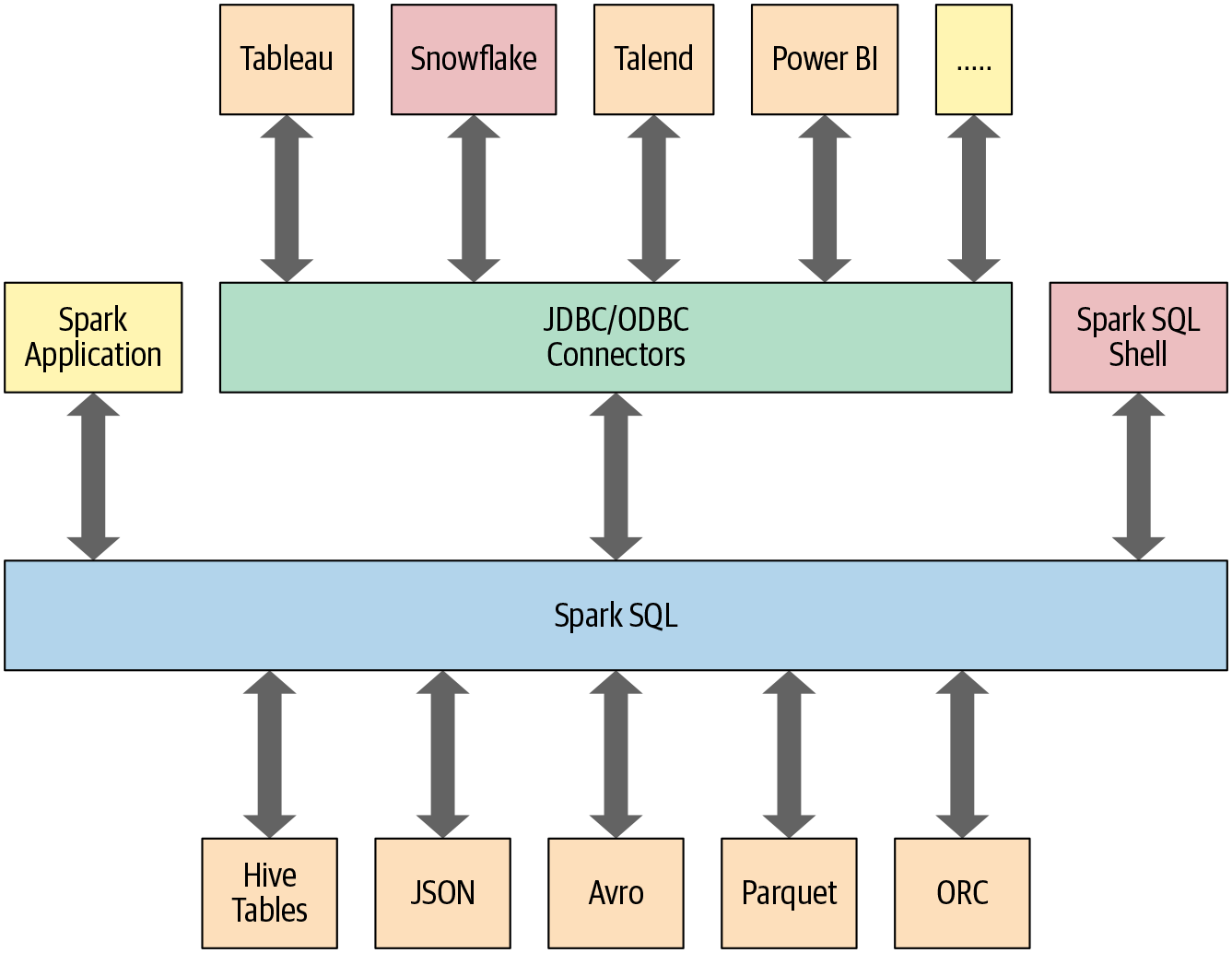
Figure 4-1. Spark SQL connectors and data sources
Let’s begin with how you can use Spark SQL in a Spark application.
Using Spark SQL in Spark Applications
The SparkSession, introduced in Spark 2.0, provides a unified entry point for programming Spark with the Structured APIs. You can use a SparkSession to access Spark functionality: just import the class and create an instance in your code.
To issue any SQL query, use the sql() method on the SparkSession instance, spark, such as spark.sql("SELECT * FROM myTableName"). All spark.sql queries executed in this manner return a DataFrame on which you may perform further Spark operations if you desire—the kind we explored in Chapter 3 and the ones you will learn about in this chapter and the next.
Basic Query Examples
In this section we’ll walk through a few examples of queries on the Airline On-Time Performance and Causes of Flight Delays data set, which contains data on US flights including date, delay, distance, origin, and destination. It’s available as a CSV file with over a million records. Using a schema, we’ll read the data into a DataFrame and register the DataFrame as a temporary view (more on temporary views shortly) so we can query it with SQL.
Query examples are provided in code snippets, and Python and Scala notebooks containing all of the code presented here are available in the book’s GitHub repo. These examples will offer you a taste of how to use SQL in your Spark applications via the spark.sql programmatic interface. Similar to the DataFrame API in its declarative flavor, this interface allows you to query structured data in your Spark applications.
Normally, in a standalone Spark application, you will create a SparkSession instance manually, as shown in the following example. However, in a Spark shell (or Databricks notebook), the SparkSession is created for you and accessible via the appropriately named variable spark.
Let’s get started by reading the data set into a temporary view:
// In Scalaimportorg.apache.spark.sql.SparkSessionvalspark=SparkSession.builder.appName("SparkSQLExampleApp").getOrCreate()// Path to data setvalcsvFile="/databricks-datasets/learning-spark-v2/flights/departuredelays.csv"// Read and create a temporary view// Infer schema (note that for larger files you may want to specify the schema)valdf=spark.read.format("csv").option("inferSchema","true").option("header","true").load(csvFile)// Create a temporary viewdf.createOrReplaceTempView("us_delay_flights_tbl")
# In Pythonfrompyspark.sqlimportSparkSession# Create a SparkSessionspark=(SparkSession.builder.appName("SparkSQLExampleApp").getOrCreate())# Path to data setcsv_file="/databricks-datasets/learning-spark-v2/flights/departuredelays.csv"# Read and create a temporary view# Infer schema (note that for larger files you# may want to specify the schema)df=(spark.read.format("csv").option("inferSchema","true").option("header","true").load(csv_file))df.createOrReplaceTempView("us_delay_flights_tbl")
Note
If you want to specify a schema, you can use a DDL-formatted string. For example:
// In Scalavalschema="date STRING, delay INT, distance INT,origin STRING, destination STRING"
# In Pythonschema="`date` STRING, `delay` INT, `distance` INT,`origin`STRING,`destination`STRING"
Now that we have a temporary view, we can issue SQL queries using Spark SQL. These queries are no different from those you might issue against a SQL table in, say, a MySQL or PostgreSQL database. The point here is to show that Spark SQL offers an ANSI:2003–compliant SQL interface, and to demonstrate the interoperability between SQL and DataFrames.
The US flight delays data set has five columns:
The
datecolumn contains a string like02190925. When converted, this maps to02-19 09:25 am.The
delaycolumn gives the delay in minutes between the scheduled and actual departure times. Early departures show negative numbers.The
distancecolumn gives the distance in miles from the origin airport to the destination airport.The
origincolumn contains the origin IATA airport code.The
destinationcolumn contains the destination IATA airport code.
With that in mind, let’s try some example queries against this data set.
First, we’ll find all flights whose distance is greater than 1,000 miles:
spark.sql("""SELECT distance, origin, destination
FROM us_delay_flights_tbl WHERE distance > 1000
ORDER BY distance DESC""").show(10)

+--------+------+-----------+
|distance|origin|destination|
+--------+------+-----------+
|4330    |HNL   |JFK        |
|4330    |HNL   |JFK        |
|4330    |HNL   |JFK        |
|4330    |HNL   |JFK        |
|4330    |HNL   |JFK        |
|4330    |HNL   |JFK        |
|4330    |HNL   |JFK        |
|4330    |HNL   |JFK        |
|4330    |HNL   |JFK        |
|4330    |HNL   |JFK        |
+--------+------+-----------+
only showing top 10 rows
As the results show, all of the longest flights were between Honolulu (HNL) and New York (JFK). Next, we’ll find all flights between San Francisco (SFO) and Chicago (ORD) with at least a two-hour delay:
spark.sql("""SELECT date, delay, origin, destination
FROM us_delay_flights_tbl
WHERE delay > 120 AND ORIGIN = 'SFO' AND DESTINATION = 'ORD'
ORDER by delay DESC""").show(10)

+--------+-----+------+-----------+
|date    |delay|origin|destination|
+--------+-----+------+-----------+
|02190925|1638 |SFO   |ORD        |
|01031755|396  |SFO   |ORD        |
|01022330|326  |SFO   |ORD        |
|01051205|320  |SFO   |ORD        |
|01190925|297  |SFO   |ORD        |
|02171115|296  |SFO   |ORD        |
|01071040|279  |SFO   |ORD        |
|01051550|274  |SFO   |ORD        |
|03120730|266  |SFO   |ORD        |
|01261104|258  |SFO   |ORD        |
+--------+-----+------+-----------+
only showing top 10 rows
It seems there were many significantly delayed flights between these two cities, on different dates. (As an exercise, convert the date column into a readable format and find the days or months when these delays were most common. Were the delays related to winter months or holidays?)
Let’s try a more complicated query where we use the CASE clause in SQL. In the following example, we want to label all US flights, regardless of origin and destination, with an indication of the delays they experienced: Very Long Delays (> 6 hours), Long Delays (2–6 hours), etc. We’ll add these human-readable labels in a new column called Flight_Delays:
spark.sql("""SELECT delay, origin, destination,
              CASE
                  WHEN delay > 360 THEN 'Very Long Delays'
                  WHEN delay >= 120 AND delay <= 360 THEN 'Long Delays'
                  WHEN delay >= 60 AND delay < 120 THEN 'Short Delays'
                  WHEN delay > 0 and delay < 60 THEN 'Tolerable Delays'
                  WHEN delay = 0 THEN 'No Delays'
                  ELSE 'Early'
               END AS Flight_Delays
               FROM us_delay_flights_tbl
               ORDER BY origin, delay DESC""").show(10)

+-----+------+-----------+-------------+
|delay|origin|destination|Flight_Delays|
+-----+------+-----------+-------------+
|333  |ABE   |ATL        |Long Delays  |
|305  |ABE   |ATL        |Long Delays  |
|275  |ABE   |ATL        |Long Delays  |
|257  |ABE   |ATL        |Long Delays  |
|247  |ABE   |DTW        |Long Delays  |
|247  |ABE   |ATL        |Long Delays  |
|219  |ABE   |ORD        |Long Delays  |
|211  |ABE   |ATL        |Long Delays  |
|197  |ABE   |DTW        |Long Delays  |
|192  |ABE   |ORD        |Long Delays  |
+-----+------+-----------+-------------+
only showing top 10 rows
As with the DataFrame and Dataset APIs, with the spark.sql interface you can conduct common data analysis operations like those we explored in the previous chapter. The computations undergo an identical journey in the Spark SQL engine (see “The Catalyst Optimizer” in Chapter 3 for details), giving you the same results.
All three of the preceding SQL queries can be expressed with an equivalent DataFrame API query. For example, the first query can be expressed in the Python DataFrame API as:
# In Pythonfrompyspark.sql.functionsimportcol,desc(df.select("distance","origin","destination").where(col("distance")>1000).orderBy(desc("distance"))).show(10)# Or(df.select("distance","origin","destination").where("distance > 1000").orderBy("distance",ascending=False).show(10))
This produces the same results as the SQL query:
+--------+------+-----------+
|distance|origin|destination|
+--------+------+-----------+
|4330    |HNL   |JFK        |
|4330    |HNL   |JFK        |
|4330    |HNL   |JFK        |
|4330    |HNL   |JFK        |
|4330    |HNL   |JFK        |
|4330    |HNL   |JFK        |
|4330    |HNL   |JFK        |
|4330    |HNL   |JFK        |
|4330    |HNL   |JFK        |
|4330    |HNL   |JFK        |
+--------+------+-----------+
only showing top 10 rows
As an exercise, try converting the other two SQL queries to use the DataFrame API.
As these examples show, using the Spark SQL interface to query data is similar to writing a regular SQL query to a relational database table. Although the queries are in SQL, you can feel the similarity in readability and semantics to DataFrame API operations, which you encountered in Chapter 3 and will explore further in the next chapter.
To enable you to query structured data as shown in the preceding examples, Spark manages all the complexities of creating and managing views and tables, both in memory and on disk. That leads us to our next topic: how tables and views are created and managed.
SQL Tables and Views
Tables hold data. Associated with each table in Spark is its relevant metadata, which is information about the table and its data: the schema, description, table name, database name, column names, partitions, physical location where the actual data resides, etc. All of this is stored in a central metastore.
Instead of having a separate metastore for Spark tables, Spark by default uses the Apache Hive metastore, located at /user/hive/warehouse, to persist all the metadata about your tables. However, you may change the default location by setting the Spark config variable spark.sql.warehouse.dir to another location, which can be set to a local or external distributed storage.
Managed Versus UnmanagedTables
Spark allows you to create two types of tables: managed and unmanaged. For a managed table, Spark manages both the metadata and the data in the file store. This could be a local filesystem, HDFS, or an object store such as Amazon S3 or Azure Blob. For an unmanaged table, Spark only manages the metadata, while you manage the data yourself in an external data source such as Cassandra.
With a managed table, because Spark manages everything, a SQL command such as DROP TABLE table_name deletes both the metadata and the data. With an unmanaged table, the same command will delete only the metadata, not the actual data. We will look at some examples of how to create managed and unmanaged tables in the next section.
Creating SQL Databases and Tables
Tables reside within a database. By default, Spark creates tables under the default database. To create your own database name, you can issue a SQL command from your Spark application or notebook. Using the US flight delays data set, let’s create both a managed and an unmanaged table. To begin, we’ll create a database called learn_spark_db and tell Spark we want to use that database:
// In Scala/Pythonspark.sql("CREATE DATABASE learn_spark_db")spark.sql("USE learn_spark_db")
From this point, any commands we issue in our application to create tables will result in the tables being created in this database and residing under the database name learn_spark_db.
Creating a managed table
To create a managed table within the database learn_spark_db, you can issue a SQL query like the following:
// In Scala/Pythonspark.sql("CREATE TABLE managed_us_delay_flights_tbl (date STRING, delay INT,distance INT, origin STRING, destination STRING)")
You can do the same thing using the DataFrame API like this:
# In Python# Path to our US flight delays CSV filecsv_file="/databricks-datasets/learning-spark-v2/flights/departuredelays.csv"# Schema as defined in the preceding exampleschema="date STRING, delay INT, distance INT, origin STRING, destination STRING"flights_df=spark.read.csv(csv_file,schema=schema)flights_df.write.saveAsTable("managed_us_delay_flights_tbl")
Both of these statements will create the managed table us_delay_flights_tbl in the learn_spark_db database.
Creating an unmanaged table
By contrast, you can create unmanaged tables from your own data sources—say, Parquet, CSV, or JSON files stored in a file store accessible to your Spark application.
To create an unmanaged table from a data source such as a CSV file, in SQL use:
spark.sql("""CREATE TABLE us_delay_flights_tbl(date STRING, delay INT,
  distance INT, origin STRING, destination STRING)
  USING csv OPTIONS (PATH
  '/databricks-datasets/learning-spark-v2/flights/departuredelays.csv')""")
And within the DataFrame API use:
(flights_df
  .write
  .option("path", "/tmp/data/us_flights_delay")
  .saveAsTable("us_delay_flights_tbl"))
Note
To enable you to explore these examples, we have created Python and Scala example notebooks that you can find in the book’s GitHub repo.
Creating Views
In addition to creating tables, Spark can create views on top of existing tables. Views can be global (visible across all SparkSessions on a given cluster) or session-scoped (visible only to a single SparkSession), and they are temporary: they disappear after your Spark application terminates.
Creating views has a similar syntax to creating tables within a database. Once you create a view, you can query it as you would a table. The difference between a view and a table is that views don’t actually hold the data; tables persist after your Spark application terminates, but views disappear.
You can create a view from an existing table using SQL. For example, if you wish to work on only the subset of the US flight delays data set with origin airports of New York (JFK) and San Francisco (SFO), the following queries will create global temporary and temporary views consisting of just that slice of the table:
-- In SQLCREATEORREPLACEGLOBALTEMPVIEWus_origin_airport_SFO_global_tmp_viewASSELECTdate,delay,origin,destinationfromus_delay_flights_tblWHEREorigin='SFO';CREATEORREPLACETEMPVIEWus_origin_airport_JFK_tmp_viewASSELECTdate,delay,origin,destinationfromus_delay_flights_tblWHEREorigin='JFK'
You can accomplish the same thing with the DataFrame API as follows:
# In Pythondf_sfo=spark.sql("SELECT date, delay, origin, destination FROMus_delay_flights_tblWHEREorigin='SFO'")df_jfk=spark.sql("SELECT date, delay, origin, destination FROMus_delay_flights_tblWHEREorigin='JFK'")# Create a temporary and global temporary viewdf_sfo.createOrReplaceGlobalTempView("us_origin_airport_SFO_global_tmp_view")df_jfk.createOrReplaceTempView("us_origin_airport_JFK_tmp_view")
Once you’ve created these views, you can issue queries against them just as you would against a table. Keep in mind that when accessing a global temporary view you must use the prefix global_temp.<view_name>, because Spark creates global temporary views in a global temporary database called global_temp. For example:
-- In SQLSELECT*FROMglobal_temp.us_origin_airport_SFO_global_tmp_view
By contrast, you can access the normal temporary view without the global_temp prefix:
-- In SQLSELECT*FROMus_origin_airport_JFK_tmp_view
// In Scala/Pythonspark.read.table("us_origin_airport_JFK_tmp_view")// Orspark.sql("SELECT * FROM us_origin_airport_JFK_tmp_view")
You can also drop a view just like you would a table:
-- In SQLDROPVIEWIFEXISTSus_origin_airport_SFO_global_tmp_view;DROPVIEWIFEXISTSus_origin_airport_JFK_tmp_view
// In Scala/Pythonspark.catalog.dropGlobalTempView("us_origin_airport_SFO_global_tmp_view")spark.catalog.dropTempView("us_origin_airport_JFK_tmp_view")
Temporary views versus global temporary views
The difference between temporary and global temporary views being subtle, it can be a source of mild confusion among developers new to Spark. A temporary view is tied to a single SparkSession within a Spark application. In contrast, a global temporary view is visible across multiple SparkSessions within a Spark application. Yes, you can create multiple SparkSessions within a single Spark application—this can be handy, for example, in cases where you want to access (and combine) data from two different SparkSessions that don’t share the same Hive metastore configurations.
Viewing the Metadata
As mentioned previously, Spark manages the metadata associated with each managed or unmanaged table. This is captured in the Catalog, a high-level abstraction in Spark SQL for storing metadata. The Catalog’s functionality was expanded in Spark 2.x with new public methods enabling you to examine the metadata associated with your databases, tables, and views. Spark 3.0 extends it to use external catalog (which we briefly discuss in Chapter 12).
For example, within a Spark application, after creating the SparkSession variable spark, you can access all the stored metadata through methods like these:
// In Scala/Pythonspark.catalog.listDatabases()spark.catalog.listTables()spark.catalog.listColumns("us_delay_flights_tbl")
Import the notebook from the book’s GitHub repo and give it a try.
Caching SQL Tables
Although we will discuss table caching strategies in the next chapter, it’s worth mentioning here that, like DataFrames, you can cache and uncache SQL tables and views. In Spark 3.0, in addition to other options, you can specify a table as LAZY, meaning that it should only be cached when it is first used instead of immediately:
-- In SQLCACHE[LAZY]TABLE<table-name>UNCACHETABLE<table-name>
Reading Tables into DataFrames
Often, data engineers build data pipelines as part of their regular data ingestion and ETL processes. They populate Spark SQL databases and tables with cleansed data for consumption by applications downstream.
Let’s assume you have an existing database, learn_spark_db, and table, us_delay_flights_tbl, ready for use. Instead of reading from an external JSON file, you can simply use SQL to query the table and assign the returned result to a DataFrame:
// In ScalavalusFlightsDF=spark.sql("SELECT * FROM us_delay_flights_tbl")valusFlightsDF2=spark.table("us_delay_flights_tbl")
# In Pythonus_flights_df=spark.sql("SELECT * FROM us_delay_flights_tbl")us_flights_df2=spark.table("us_delay_flights_tbl")
Now you have a cleansed DataFrame read from an existing Spark SQL table. You can also read data in other formats using Spark’s built-in data sources, giving you the flexibility to interact with various common file formats.
Data Sources for DataFrames and SQL Tables
As shown in Figure 4-1, Spark SQL provides an interface to a variety of data sources. It also provides a set of common methods for reading and writing data to and from these data sources using the Data Sources API.
In this section we will cover some of the built-in data sources, available file formats, and ways to load and write data, along with specific options pertaining to these data sources. But first, let’s take a closer look at two high-level Data Source API constructs that dictate the manner in which you interact with different data sources: DataFrameReader and DataFrameWriter.
DataFrameReader
DataFrameReader is the core construct for reading data from a data source into a DataFrame. It has a defined format and a recommended pattern for usage:
DataFrameReader.format(args).option("key", "value").schema(args).load()
This pattern of stringing methods together is common in Spark, and easy to read. We saw it in Chapter 3 when exploring common data analysis patterns.
Note that you can only access a DataFrameReader through a SparkSession instance. That is, you cannot create an instance of DataFrameReader. To get an instance handle to it, use:
SparkSession.read
// or
SparkSession.readStream
While read returns a handle to DataFrameReader to read into a DataFrame from a static data source, readStream returns an instance to read from a streaming source. (We will cover Structured Streaming later in the book.)
Arguments to each of the public methods to DataFrameReader take different values. Table 4-1 enumerates these, with a subset of the supported arguments.
| Method | Arguments | Description |
|---|---|---|
format() |
"parquet", "csv", "txt", "json", "jdbc", "orc", "avro", etc. |
If you don’t specify this method, then the default is Parquet or whatever is set in spark.sql.sources.default. |
option() |
("mode", {PERMISSIVE | FAILFAST | DROPMALFORMED } )("inferSchema", {true | false})("path", "path_file_data_source") |
A series of key/value pairs and options. The Spark documentation shows some examples and explains the different modes and their actions. The default mode is PERMISSIVE. The "inferSchema" and "mode" options are specific to the JSON and CSV file formats. |
schema() |
DDL String or StructType, e.g., 'A INT, B STRING' orStructType(...) |
For JSON or CSV format, you can specify to infer the schema in the option() method. Generally, providing a schema for any format makes loading faster and ensures your data conforms to the expected schema. |
load() |
"/path/to/data/source" |
The path to the data source. This can be empty if specified in option("path", "..."). |
While we won’t comprehensively enumerate all the different combinations of arguments and options, the documentation for Python, Scala, R, and Java offers suggestions and guidance. It’s worthwhile to show a couple of examples, though:
// In Scala// Use Parquetvalfile="""/databricks-datasets/learning-spark-v2/flights/summary-data/parquet/2010-summary.parquet"""valdf=spark.read.format("parquet").load(file)// Use Parquet; you can omit format("parquet") if you wish as it's the defaultvaldf2=spark.read.load(file)// Use CSVvaldf3=spark.read.format("csv").option("inferSchema","true").option("header","true").option("mode","PERMISSIVE").load("/databricks-datasets/learning-spark-v2/flights/summary-data/csv/*")// Use JSONvaldf4=spark.read.format("json").load("/databricks-datasets/learning-spark-v2/flights/summary-data/json/*")
Note
In general, no schema is needed when reading from a static Parquet data source—the Parquet metadata usually contains the schema, so it’s inferred. However, for streaming data sources you will have to provide a schema. (We will cover reading from streaming data sources in Chapter 8.)
Parquet is the default and preferred data source for Spark because it’s efficient, uses columnar storage, and employs a fast compression algorithm. You will see additional benefits later (such as columnar pushdown), when we cover the Catalyst optimizer in greater depth.
DataFrameWriter
DataFrameWriter does the reverse of its counterpart: it saves or writes data to a specified built-in data source. Unlike with DataFrameReader, you access its instance not from a SparkSession but from the DataFrame you wish to save. It has a few recommended usage patterns:
DataFrameWriter.format(args)
  .option(args)
  .bucketBy(args)
  .partitionBy(args)
  .save(path)

DataFrameWriter.format(args).option(args).sortBy(args).saveAsTable(table)
To get an instance handle, use:
DataFrame.write
// or
DataFrame.writeStream
Arguments to each of the methods to DataFrameWriter also take different values. We list these in Table 4-2, with a subset of the supported arguments.
| Method | Arguments | Description |
|---|---|---|
format() |
"parquet", "csv", "txt", "json", "jdbc", "orc", "avro", etc. |
If you don’t specify this method, then the default is Parquet or whatever is set in spark.sql.sources.default. |
option() |
("mode", {append | overwrite | ignore | error or errorifexists} )("mode", {SaveMode.Overwrite | SaveMode.Append, SaveMode.Ignore, SaveMode.ErrorIfExists})("path", "path_to_write_to") |
A series of key/value pairs and options. The Spark documentation shows some examples. This is an overloaded method. The default mode options are error or errorifexists and SaveMode.ErrorIfExists; they throw an exception at runtime if the data already exists. |
bucketBy() |
(numBuckets, col, col..., coln) |
The number of buckets and names of columns to bucket by. Uses Hive’s bucketing scheme on a filesystem. |
save()
|
"/path/to/data/source" |
The path to save to. This can be empty if specified in option("path", "..."). |
saveAsTable() |
"table_name" |
The table to save to. |
Here’s a short example snippet to illustrate the use of methods and arguments:
// In Scala// Use JSONvallocation=...df.write.format("json").mode("overwrite").save(location)
Parquet
We’ll start our exploration of data sources with Parquet, because it’s the default data source in Spark. Supported and widely used by many big data processing frameworks and platforms, Parquet is an open source columnar file format that offers many I/O optimizations (such as compression, which saves storage space and allows for quick access to data columns).
Because of its efficiency and these optimizations, we recommend that after you have transformed and cleansed your data, you save your DataFrames in the Parquet format for downstream consumption. (Parquet is also the default table open format for Delta Lake, which we will cover in Chapter 9.)
Reading Parquet files into a DataFrame
Parquet files are stored in a directory structure that contains the data files, metadata, a number of compressed files, and some status files. Metadata in the footer contains the version of the file format, the schema, and column data such as the path, etc.
For example, a directory in a Parquet file might contain a set of files like this:
_SUCCESS
_committed_1799640464332036264
_started_1799640464332036264
part-00000-tid-1799640464332036264-91273258-d7ef-4dc7-<...>-c000.snappy.parquet
There may be a number of part-XXXX compressed files in a directory (the names shown here have been shortened to fit on the page).
To read Parquet files into a DataFrame, you simply specify the format and path:
// In Scalavalfile="""/databricks-datasets/learning-spark-v2/flights/summary-data/parquet/2010-summary.parquet/"""valdf=spark.read.format("parquet").load(file)
# In Pythonfile="""/databricks-datasets/learning-spark-v2/flights/summary-data/parquet/2010-summary.parquet/"""df=spark.read.format("parquet").load(file)
Unless you are reading from a streaming data source there’s no need to supply the schema, because Parquet saves it as part of its metadata.
Reading Parquet files into a Spark SQL table
As well as reading Parquet files into a Spark DataFrame, you can also create a Spark SQL unmanaged table or view directly using SQL:
-- In SQLCREATEORREPLACETEMPORARYVIEWus_delay_flights_tblUSINGparquetOPTIONS(path"/databricks-datasets/learning-spark-v2/flights/summary-data/parquet/2010-summary.parquet/")
Once you’ve created the table or view, you can read data into a DataFrame using SQL, as we saw in some earlier examples:
// In Scalaspark.sql("SELECT * FROM us_delay_flights_tbl").show()
# In Pythonspark.sql("SELECT * FROM us_delay_flights_tbl").show()
Both of these operations return the same results:
+-----------------+-------------------+-----+
|DEST_COUNTRY_NAME|ORIGIN_COUNTRY_NAME|count|
+-----------------+-------------------+-----+
|United States    |Romania            |1    |
|United States    |Ireland            |264  |
|United States    |India              |69   |
|Egypt            |United States      |24   |
|Equatorial Guinea|United States      |1    |
|United States    |Singapore          |25   |
|United States    |Grenada            |54   |
|Costa Rica       |United States      |477  |
|Senegal          |United States      |29   |
|United States    |Marshall Islands   |44   |
+-----------------+-------------------+-----+
only showing top 10 rows
Writing DataFrames to Parquet files
Writing or saving a DataFrame as a table or file is a common operation in Spark. To write a DataFrame you simply use the methods and arguments to the DataFrameWriter outlined earlier in this chapter, supplying the location to save the Parquet files to. For example:
// In Scaladf.write.format("parquet").mode("overwrite").option("compression","snappy").save("/tmp/data/parquet/df_parquet")
# In Python(df.write.format("parquet").mode("overwrite").option("compression","snappy").save("/tmp/data/parquet/df_parquet"))
Note
Recall that Parquet is the default file format. If you don’t include the format() method, the DataFrame will still be saved as a Parquet file.
This will create a set of compact and compressed Parquet files at the specified path. Since we used snappy as our compression choice here, we’ll have snappy compressed files. For brevity, this example generated only one file; normally, there may be a dozen or so files created:
-rw-r--r--  1 jules  wheel    0 May 19 10:58 _SUCCESS
-rw-r--r--  1 jules  wheel  966 May 19 10:58 part-00000-<...>-c000.snappy.parquet
Writing DataFrames to Spark SQL tables
Writing a DataFrame to a SQL table is as easy as writing to a file—just use saveAsTable() instead of save(). This will create a managed table called us_delay_flights_tbl:
// In Scaladf.write.mode("overwrite").saveAsTable("us_delay_flights_tbl")
# In Python(df.write.mode("overwrite").saveAsTable("us_delay_flights_tbl"))
To sum up, Parquet is the preferred and default built-in data source file format in Spark, and it has been adopted by many other frameworks. We recommend that you use this format in your ETL and data ingestion processes.
JSON
JavaScript Object Notation (JSON) is also a popular data format. It came to prominence as an easy-to-read and easy-to-parse format compared to XML. It has two representational formats: single-line mode and multiline mode. Both modes are supported in Spark.
In single-line mode each line denotes a single JSON object, whereas in multiline mode the entire multiline object constitutes a single JSON object. To read in this mode, set multiLine to true in the option() method.
Reading a JSON file into a DataFrame
You can read a JSON file into a DataFrame the same way you did with Parquet—just specify "json" in the format() method:
// In Scalavalfile="/databricks-datasets/learning-spark-v2/flights/summary-data/json/*"valdf=spark.read.format("json").load(file)
# In Pythonfile="/databricks-datasets/learning-spark-v2/flights/summary-data/json/*"df=spark.read.format("json").load(file)
Reading a JSON file into a Spark SQL table
You can also create a SQL table from a JSON file just like you did with Parquet:
-- In SQLCREATEORREPLACETEMPORARYVIEWus_delay_flights_tblUSINGjsonOPTIONS(path"/databricks-datasets/learning-spark-v2/flights/summary-data/json/*")
Once the table is created, you can read data into a DataFrame using SQL:
//InScala/Pythonspark.sql("SELECT * FROM us_delay_flights_tbl").show()+-----------------+-------------------+-----+|DEST_COUNTRY_NAME|ORIGIN_COUNTRY_NAME|count|+-----------------+-------------------+-----+|UnitedStates|Romania|15||UnitedStates|Croatia|1||UnitedStates|Ireland|344||Egypt|UnitedStates|15||UnitedStates|India|62||UnitedStates|Singapore|1||UnitedStates|Grenada|62||CostaRica|UnitedStates|588||Senegal|UnitedStates|40||Moldova|UnitedStates|1|+-----------------+-------------------+-----+onlyshowingtop10rows
Writing DataFrames to JSON files
Saving a DataFrame as a JSON file is simple. Specify the appropriate DataFrameWriter methods and arguments, and supply the location to save the JSON files to:
// In Scaladf.write.format("json").mode("overwrite").option("compression","snappy").save("/tmp/data/json/df_json")
# In Python(df.write.format("json").mode("overwrite").option("compression","snappy").save("/tmp/data/json/df_json"))
This creates a directory at the specified path populated with a set of compact JSON files:
-rw-r--r--  1 jules  wheel   0 May 16 14:44 _SUCCESS
-rw-r--r--  1 jules  wheel  71 May 16 14:44 part-00000-<...>-c000.json
JSON data source options
Table 4-3 describes common JSON options for DataFrameReader and DataFrameWriter. For a comprehensive list, we refer you to the documentation.
| Property name | Values | Meaning | Scope |
|---|---|---|---|
compression |
none, uncompressed, bzip2, deflate, gzip, lz4, or snappy |
Use this compression codec for writing. Note that read will only detect the compression or codec from the file extension. | Write |
dateFormat |
yyyy-MM-dd or DateTimeFormatter |
Use this format or any format from Java’s DateTimeFormatter. |
Read/write |
multiLine |
true, false |
Use multiline mode. Default is false (single-line mode). |
Read |
allowUnquotedFieldNames |
true, false |
Allow unquoted JSON field names. Default is false. |
Read |
CSV
As widely used as plain text files, this common text file format captures each datum or field delimited by a comma; each line with comma-separated fields represents a record. Even though a comma is the default separator, you may use other delimiters to separate fields in cases where commas are part of your data. Popular spreadsheets can generate CSV files, so it’s a popular format among data and business analysts.
Reading a CSV file into a DataFrame
As with the other built-in data sources, you can use the DataFrameReader methods and arguments to read a CSV file into a DataFrame:
// In Scalavalfile="/databricks-datasets/learning-spark-v2/flights/summary-data/csv/*"valschema="DEST_COUNTRY_NAME STRING, ORIGIN_COUNTRY_NAME STRING, count INT"valdf=spark.read.format("csv").schema(schema).option("header","true").option("mode","FAILFAST")// Exit if any errors.option("nullValue","")// Replace any null data with quotes.load(file)
# In Pythonfile="/databricks-datasets/learning-spark-v2/flights/summary-data/csv/*"schema="DEST_COUNTRY_NAME STRING, ORIGIN_COUNTRY_NAME STRING, count INT"df=(spark.read.format("csv").option("header","true").schema(schema).option("mode","FAILFAST")# Exit if any errors.option("nullValue","")# Replace any null data field with quotes.load(file))
Reading a CSV file into a Spark SQL table
Creating a SQL table from a CSV data source is no different from using Parquet or JSON:
-- In SQLCREATEORREPLACETEMPORARYVIEWus_delay_flights_tblUSINGcsvOPTIONS(path"/databricks-datasets/learning-spark-v2/flights/summary-data/csv/*",header"true",inferSchema"true",mode"FAILFAST")
Once you’ve created the table, you can read data into a DataFrame using SQL as before:
//InScala/Pythonspark.sql("SELECT * FROM us_delay_flights_tbl").show(10)+-----------------+-------------------+-----+|DEST_COUNTRY_NAME|ORIGIN_COUNTRY_NAME|count|+-----------------+-------------------+-----+|UnitedStates|Romania|1||UnitedStates|Ireland|264||UnitedStates|India|69||Egypt|UnitedStates|24||EquatorialGuinea|UnitedStates|1||UnitedStates|Singapore|25||UnitedStates|Grenada|54||CostaRica|UnitedStates|477||Senegal|UnitedStates|29||UnitedStates|MarshallIslands|44|+-----------------+-------------------+-----+onlyshowingtop10rows
Writing DataFrames to CSV files
Saving a DataFrame as a CSV file is simple. Specify the appropriate DataFrameWriter methods and arguments, and supply the location to save the CSV files to:
// In Scaladf.write.format("csv").mode("overwrite").save("/tmp/data/csv/df_csv")
# In Pythondf.write.format("csv").mode("overwrite").save("/tmp/data/csv/df_csv")
This generates a folder at the specified location, populated with a bunch of compressed and compact files:
-rw-r--r--  1 jules  wheel   0 May 16 12:17 _SUCCESS
-rw-r--r--  1 jules  wheel  36 May 16 12:17 part-00000-251690eb-<...>-c000.csv
CSV data source options
Table 4-4 describes some of the common CSV options for DataFrameReader and DataFrameWriter. Because CSV files can be complex, many options are available; for a comprehensive list we refer you to the documentation.
| Property name | Values | Meaning | Scope |
|---|---|---|---|
compression |
none, bzip2, deflate, gzip, lz4, or snappy |
Use this compression codec for writing. | Write |
dateFormat |
yyyy-MM-dd or DateTimeFormatter |
Use this format or any format from Java’s DateTimeFormatter. |
Read/write |
multiLine |
true, false |
Use multiline mode. Default is false (single-line mode). |
Read |
inferSchema |
true, false |
If true, Spark will determine the column data types. Default is false. |
Read |
sep |
Any character | Use this character to separate column values in a row. Default delimiter is a comma (,). |
Read/write |
escape |
Any character | Use this character to escape quotes. Default is \. |
Read/write |
header |
true, false |
Indicates whether the first line is a header denoting each column name. Default is false. |
Read/write |
Avro
Introduced in Spark 2.4 as a built-in data source, the Avro format is used, for example, by Apache Kafka for message serializing and deserializing. It offers many benefits, including direct mapping to JSON, speed and efficiency, and bindings available for many programming languages.
Reading an Avro file into a DataFrame
Reading an Avro file into a DataFrame using DataFrameReader is consistent in usage with the other data sources we have discussed in this section:
// In Scalavaldf=spark.read.format("avro").load("/databricks-datasets/learning-spark-v2/flights/summary-data/avro/*")df.show(false)
# In Pythondf=(spark.read.format("avro").load("/databricks-datasets/learning-spark-v2/flights/summary-data/avro/*"))df.show(truncate=False)+-----------------+-------------------+-----+|DEST_COUNTRY_NAME|ORIGIN_COUNTRY_NAME|count|+-----------------+-------------------+-----+|UnitedStates|Romania|1||UnitedStates|Ireland|264||UnitedStates|India|69||Egypt|UnitedStates|24||EquatorialGuinea|UnitedStates|1||UnitedStates|Singapore|25||UnitedStates|Grenada|54||CostaRica|UnitedStates|477||Senegal|UnitedStates|29||UnitedStates|MarshallIslands|44|+-----------------+-------------------+-----+onlyshowingtop10rows
Reading an Avro file into a Spark SQL table
Again, creating SQL tables using an Avro data source is no different from using Parquet, JSON, or CSV:
-- In SQLCREATEORREPLACETEMPORARYVIEWepisode_tblUSINGavroOPTIONS(path"/databricks-datasets/learning-spark-v2/flights/summary-data/avro/*")
Once you’ve created a table, you can read data into a DataFrame using SQL:
// In Scalaspark.sql("SELECT * FROM episode_tbl").show(false)
# In Pythonspark.sql("SELECT * FROM episode_tbl").show(truncate=False)+-----------------+-------------------+-----+|DEST_COUNTRY_NAME|ORIGIN_COUNTRY_NAME|count|+-----------------+-------------------+-----+|UnitedStates|Romania|1||UnitedStates|Ireland|264||UnitedStates|India|69||Egypt|UnitedStates|24||EquatorialGuinea|UnitedStates|1||UnitedStates|Singapore|25||UnitedStates|Grenada|54||CostaRica|UnitedStates|477||Senegal|UnitedStates|29||UnitedStates|MarshallIslands|44|+-----------------+-------------------+-----+onlyshowingtop10rows
Writing DataFrames to Avro files
Writing a DataFrame as an Avro file is simple. As usual, specify the appropriate DataFrameWriter methods and arguments, and supply the location to save the Avro files to:
// In Scaladf.write.format("avro").mode("overwrite").save("/tmp/data/avro/df_avro")
# In Python(df.write.format("avro").mode("overwrite").save("/tmp/data/avro/df_avro"))
This generates a folder at the specified location, populated with a bunch of compressed and compact files:
-rw-r--r--  1 jules  wheel    0 May 17 11:54 _SUCCESS
-rw-r--r--  1 jules  wheel  526 May 17 11:54 part-00000-ffdf70f4-<...>-c000.avro
Avro data source options
Table 4-5 describes common options for DataFrameReader and DataFrameWriter. A comprehensive list of options is in the documentation.
| Property name | Default value | Meaning | Scope |
|---|---|---|---|
avroSchema |
None | Optional Avro schema provided by a user in JSON format. The data type and naming of record fields should match the input Avro data or Catalyst data (Spark internal data type), otherwise the read/write action will fail. | Read/write |
recordName |
topLevelRecord |
Top-level record name in write result, which is required in the Avro spec. | Write |
recordNamespace |
"" |
Record namespace in write result. | Write |
ignoreExtension |
true |
If this option is enabled, all files (with and without the .avro extension) are loaded. Otherwise, files without the .avro extension are ignored. | Read |
compression |
snappy |
Allows you to specify the compression codec to use in writing. Currently supported codecs are uncompressed, snappy, deflate, bzip2, and xz.If this option is not set, the value in spark.sql.avro.compression.codec is taken into account. |
Write |
ORC
As an additional optimized columnar file format, Spark 2.x supports a vectorized ORC reader. Two Spark configurations dictate which ORC implementation to use. When spark.sql.orc.impl is set to native and spark.sql.orc.enableVectorizedReader is set to true, Spark uses the vectorized ORC reader. A vectorized reader reads blocks of rows (often 1,024 per block) instead of one row at a time, streamlining operations and reducing CPU usage for intensive operations like scans, filters, aggregations, and joins.
For Hive ORC SerDe (serialization and deserialization) tables created with the SQL command USING HIVE OPTIONS (fileFormat 'ORC'), the vectorized reader is used when the Spark configuration parameter spark.sql.hive.convertMetastoreOrc is set to true.
Reading an ORC file into a DataFrame
To read in a DataFrame using the ORC vectorized reader, you can just use the normal DataFrameReader methods and options:
// In Scalavalfile="/databricks-datasets/learning-spark-v2/flights/summary-data/orc/*"valdf=spark.read.format("orc").load(file)df.show(10,false)
# In Pythonfile="/databricks-datasets/learning-spark-v2/flights/summary-data/orc/*"df=spark.read.format("orc").option("path",file).load()df.show(10,False)+-----------------+-------------------+-----+|DEST_COUNTRY_NAME|ORIGIN_COUNTRY_NAME|count|+-----------------+-------------------+-----+|UnitedStates|Romania|1||UnitedStates|Ireland|264||UnitedStates|India|69||Egypt|UnitedStates|24||EquatorialGuinea|UnitedStates|1||UnitedStates|Singapore|25||UnitedStates|Grenada|54||CostaRica|UnitedStates|477||Senegal|UnitedStates|29||UnitedStates|MarshallIslands|44|+-----------------+-------------------+-----+onlyshowingtop10rows
Reading an ORC file into a Spark SQL table
There is no difference from Parquet, JSON, CSV, or Avro when creating a SQL view using an ORC data source:
-- In SQLCREATEORREPLACETEMPORARYVIEWus_delay_flights_tblUSINGorcOPTIONS(path"/databricks-datasets/learning-spark-v2/flights/summary-data/orc/*")
Once a table is created, you can read data into a DataFrame using SQL as usual:
//InScala/Pythonspark.sql("SELECT * FROM us_delay_flights_tbl").show()+-----------------+-------------------+-----+|DEST_COUNTRY_NAME|ORIGIN_COUNTRY_NAME|count|+-----------------+-------------------+-----+|UnitedStates|Romania|1||UnitedStates|Ireland|264||UnitedStates|India|69||Egypt|UnitedStates|24||EquatorialGuinea|UnitedStates|1||UnitedStates|Singapore|25||UnitedStates|Grenada|54||CostaRica|UnitedStates|477||Senegal|UnitedStates|29||UnitedStates|MarshallIslands|44|+-----------------+-------------------+-----+onlyshowingtop10rows
Writing DataFrames to ORC files
Writing back a transformed DataFrame after reading is equally simple using the DataFrameWriter methods:
// In Scaladf.write.format("orc").mode("overwrite").option("compression","snappy").save("/tmp/data/orc/df_orc")
# In Python(df.write.format("orc").mode("overwrite").option("compression","snappy").save("/tmp/data/orc/flights_orc"))
The result will be a folder at the specified location containing some compressed ORC files:
-rw-r--r--  1 jules  wheel    0 May 16 17:23 _SUCCESS
-rw-r--r--  1 jules  wheel  547 May 16 17:23 part-00000-<...>-c000.snappy.orc
Images
In Spark 2.4 the community introduced a new data source, image files, to support deep learning and machine learning frameworks such as TensorFlow and PyTorch. For computer vision–based machine learning applications, loading and processing image data sets is important.
Reading an image file into a DataFrame
As with all of the previous file formats, you can use the DataFrameReader methods and options to read in an image file as shown here:
// In Scalaimportorg.apache.spark.ml.source.imagevalimageDir="/databricks-datasets/learning-spark-v2/cctvVideos/train_images/"valimagesDF=spark.read.format("image").load(imageDir)imagesDF.printSchemaimagesDF.select("image.height","image.width","image.nChannels","image.mode","label").show(5,false)
# In Pythonfrompyspark.mlimportimageimage_dir="/databricks-datasets/learning-spark-v2/cctvVideos/train_images/"images_df=spark.read.format("image").load(image_dir)images_df.printSchema()root|--image:struct(nullable=true)||--origin:string(nullable=true)||--height:integer(nullable=true)||--width:integer(nullable=true)||--nChannels:integer(nullable=true)||--mode:integer(nullable=true)||--data:binary(nullable=true)|--label:integer(nullable=true)images_df.select("image.height","image.width","image.nChannels","image.mode","label").show(5,truncate=False)+------+-----+---------+----+-----+|height|width|nChannels|mode|label|+------+-----+---------+----+-----+|288|384|3|16|0||288|384|3|16|1||288|384|3|16|0||288|384|3|16|0||288|384|3|16|0|+------+-----+---------+----+-----+onlyshowingtop5rows
Binary Files
Spark 3.0 adds support for binary files as a data source. The DataFrameReader converts each binary file into a single DataFrame row (record) that contains the raw content and metadata of the file. The binary file data source produces a DataFrame with the following columns:
path: StringType
modificationTime: TimestampType
length: LongType
content: BinaryType
Reading a binary file into a DataFrame
To read binary files, specify the data source format as a binaryFile. You can load files with paths matching a given global pattern while preserving the behavior of partition discovery with the data source option pathGlobFilter. For example, the following code reads all JPG files from the input directory with any partitioned directories:
// In Scalavalpath="/databricks-datasets/learning-spark-v2/cctvVideos/train_images/"valbinaryFilesDF=spark.read.format("binaryFile").option("pathGlobFilter","*.jpg").load(path)binaryFilesDF.show(5)
# In Pythonpath="/databricks-datasets/learning-spark-v2/cctvVideos/train_images/"binary_files_df=(spark.read.format("binaryFile").option("pathGlobFilter","*.jpg").load(path))binary_files_df.show(5)+--------------------+-------------------+------+--------------------+-----+|path|modificationTime|length|content|label|+--------------------+-------------------+------+--------------------+-----+|file:/Users/jules...|2020-02-1212:04:24|55037|[FFD8FFE0001...|0||file:/Users/jules...|2020-02-1212:04:24|54634|[FFD8FFE0001...|1||file:/Users/jules...|2020-02-1212:04:24|54624|[FFD8FFE0001...|0||file:/Users/jules...|2020-02-1212:04:24|54505|[FFD8FFE0001...|0||file:/Users/jules...|2020-02-1212:04:24|54475|[FFD8FFE0001...|0|+--------------------+-------------------+------+--------------------+-----+onlyshowingtop5rows
To ignore partitioning data discovery in a directory, you can set recursiveFileLookup to "true":
// In ScalavalbinaryFilesDF=spark.read.format("binaryFile").option("pathGlobFilter","*.jpg").option("recursiveFileLookup","true").load(path)binaryFilesDF.show(5)
# In Pythonbinary_files_df=(spark.read.format("binaryFile").option("pathGlobFilter","*.jpg").option("recursiveFileLookup","true").load(path))binary_files_df.show(5)+--------------------+-------------------+------+--------------------+|path|modificationTime|length|content|+--------------------+-------------------+------+--------------------+|file:/Users/jules...|2020-02-1212:04:24|55037|[FFD8FFE0001...||file:/Users/jules...|2020-02-1212:04:24|54634|[FFD8FFE0001...||file:/Users/jules...|2020-02-1212:04:24|54624|[FFD8FFE0001...||file:/Users/jules...|2020-02-1212:04:24|54505|[FFD8FFE0001...||file:/Users/jules...|2020-02-1212:04:24|54475|[FFD8FFE0001...|+--------------------+-------------------+------+--------------------+onlyshowingtop5rows
Note that the label column is absent when the recursiveFileLookup option is set to "true".
Currently, the binary file data source does not support writing a DataFrame back to the original file format.
In this section, you got a tour of how to read data into a DataFrame from a range of supported file formats. We also showed you how to create temporary views and tables from the existing built-in data sources. Whether you’re using the DataFrame API or SQL, the queries produce identical outcomes. You can examine some of these queries in the notebook available in the GitHub repo for this book.
Summary
To recap, this chapter explored the interoperability between the DataFrame API and Spark SQL. In particular, you got a flavor of how to use Spark SQL to:
Create managed and unmanaged tables using Spark SQL and the DataFrame API.
Read from and write to various built-in data sources and file formats.
Employ the
spark.sqlprogrammatic interface to issue SQL queries on structured data stored as Spark SQL tables or views.Peruse the Spark
Catalogto inspect metadata associated with tables and views.Use the
DataFrameWriterandDataFrameReaderAPIs.
Through the code snippets in the chapter and the notebooks available in the book’s GitHub repo, you got a feel for how to use DataFrames and Spark SQL. Continuing in this vein, the next chapter further explores how Spark interacts with the external data sources shown in Figure 4-1. You’ll see some more in-depth examples of transformations and the interoperability between the DataFrame API and Spark SQL.
Get Learning Spark, 2nd Edition now with the O’Reilly learning platform.
O’Reilly members experience books, live events, courses curated by job role, and more from O’Reilly and nearly 200 top publishers.

