Mastering Algorithms with Perl

Chapter 1.  Introduction

Computer Science is no more about computers than astronomy is about telescopes.

—E. W. Dijkstra

In this chapter, we’ll discuss how to “think algorithms”—how to design and analyze programs that solve problems. We’ll start with a gentle introduction to algorithms and a not-so-gentle introduction to Perl, then consider some of the tradeoffs involved in choosing the right implementation for your needs, and finally introduce some themes pervading the field: recursion, divide-and-conquer, and dynamic programming.

What Is an Algorithm?

An algorithm is simply a technique—not necessarily computational—for solving a problem step by step. Of course, all programs solve problems (except for the ones that create problems). What elevates some techniques to the hallowed status of algorithm is that they embody a general, reusable method that solves an entire class of problems. Programs are created; algorithms are invented. Programs eventually become obsolete; algorithms are permanent.

Of course, some algorithms are better than others. Consider the task of finding a word in a dictionary. Whether it’s a physical book or an online file containing one word per line, there are different ways to locate the word you’re looking for. You could look up a definition with a linear search, by reading the dictionary from front to back until you happen across your word. That’s slow, unless your word happens to be at the very beginning of the alphabet. Or, you could pick pages at random and scan them for your word. You might get lucky. Still, there’s obviously a better way. That better way is the binary search algorithm, which you’ll learn about in Chapter 5. In fact, the binary search is provably the best algorithm for this task.

A Sample Algorithm: Binary Search

We’ll use binary search to explore what an algorithm is, how we implement one in Perl, and what it means for an algorithm to be general and efficient. In what follows, we’ll assume that we have an alphabetically ordered list of words, and we want to determine where our chosen word appears in the list, if it even appears at all. In our program, each word is represented in Perl as a scalar, which can be an integer, a floating-point number, or (as in this case) a string of characters. Our list of words is stored in a Perl array: an ordered list of scalars. In Perl, all scalars begin with an $ sign, and all arrays begin with an @ sign. The other common datatype in Perl is the hash, denoted with a % sign. Hashes “map” one set of scalars (the “keys”) to other scalars (the “values”).

Here’s how our binary search works. At all times, there is a range of words, called a window, that the algorithm is considering. If the word is in the list, it must be inside the window. Initially, the window is the entire list: no surprise there. As the algorithm operates, it shrinks the window. Sometimes it moves the top of the window down, and sometimes it moves the bottom of the window up. Eventually, the window contains only the target word, or it contains nothing at all and we know that the word must not be in the list.

The window is defined with two numbers: the lowest and highest locations (which we’ll call indices, since we’re searching through an array) where the word might be found. Initially, the window is the entire array, since the word could be anywhere. The lower bound of the window is $low, and the higher bound is $high.

We then look at the word in the middle of the window; that is, the element with index ($low + $high) / 2. However, that expression might have a fractional value, so we wrap it in an int() to ensure that we have an integer, yielding int(($low + $high) / 2). If that word comes after our word alphabetically, we can decrease $high to this index. Likewise, if the word is too low, we increase $low to this index.

Eventually, we’ll end up with our word—or an empty window, in which case our subroutine returns undef to signal that the word isn’t present.

Before we show you the Perl program for binary search, let’s first look at how this might be written in other algorithm books. Here’s a pseudocode “implementation” of binary search:

BINARY-SEARCH(A, w)
1. low ← 0
2. high ← length[A]
3. while low < high
4. do  try ← int ((low + high) / 2)
5.    if   A[try] > w
6.    then high ← try
7.    else if   A[try] < w
8.         then low ← try + 1
9.         else return try
10.        end if
11.   end if
12. end do
13. return NO_ELEMENT

And now the Perl program. Not only is it shorter, it’s an honest-to-goodness working subroutine.

# $index = binary_search( \@array, $word )
#   @array is a list of lowercase strings in alphabetical order.
#   $word is the target word that might be in the list.
#   binary_search() returns the array index such that $array[$index]
#   is $word.

sub binary_search {
    my ($array, $word) = @_;
    my ($low, $high) = ( 0, @$array - 1 );

    while ( $low <= $high ) {              # While the window is open
        my $try = int( ($low+$high)/2 );      # Try the middle element
        $low  = $try+1, next if $array->[$try] lt $word; # Raise bottom
        $high = $try-1, next if $array->[$try] gt $word; # Lower top

        return $try;     # We've found the word!
    }
    return;              # The word isn't there.
}

Depending on how much Perl you know, this might seem crystal clear or hopelessly opaque. As the preface said, if you don’t know Perl, you probably don’t want to learn it with this book. Nevertheless, here’s a brief description of the Perl syntax used in the binary_search() subroutine.

What do all those funny symbols mean?

What you’ve just seen is the definition of a subroutine, which by itself won’t do anything. You use it by including the subroutine in your program and then providing it with the two parameters it needs: \@array and $word. \@array is a reference to the array named @array.

The first line, sub binary_search {, begins the definition of the subroutine named “binary_search”. That definition ends with the closing brace } at the very end of the code.

Next, my ($array, $word) = @_;, assigns the first two subroutine arguments to the scalars $array and $word. You know they’re scalars because they begin with dollar signs. The my statement declares the scope of the variables—they’re lexical variables, private to this subroutine, and will vanish when the subroutine finishes. Use my whenever you can.

The following line, my ($low, $high) = ( 0, @$array - 1 ); declares and initializes two more lexical scalars. $low is initialized to 0—actually unnecessary, but good form. $high is initialized to @$array - 1, which dereferences the scalar variable $array to get at the array underneath. In this context, the statement computes the length (@$array) and subtracts 1 to get the index of the last element.

Hopefully, the first argument passed to binary_search() was a reference to an array. Thanks to the first my line of the subroutine, that reference is now accessible as $array, and the array pointed to by that value can be accessed as @$array.

Then the subroutine enters a while loop, which executes as long as $low <= $high; that is, as long as our window is still open. Inside the loop, the word to be checked (more precisely, the index of the word to be checked) is assigned to $try. If that word precedes our target word,^[1] we assign $try + 1 to $low, which shrinks the window to include only the elements following $try, and we jump back to the beginning of the while loop via the next. If our target word precedes the current word, we adjust $high instead. If neither word precedes the other, we have a match, and we return $try. If our while loop exits, we know that the word isn’t present, and so undef is returned.

References

The most significant addition to the Perl language in Perl 5 is references; their use is described in the perlref documentation bundled with Perl. A reference is a scalar value (thus, all references begin with a $) whose value is the location (more or less) of another variable. That variable might be another scalar, or an array, a hash, or even a snippet of Perl code. The advantage of references is that they provide a level of indirection. Whenever you invoke a subroutine, Perl needs to copy the subroutine arguments. If you pass an array of ten thousand elements, those all have to be copied. But if you pass a reference to those elements as we’ve done in binary_search(), only the reference needs to be copied. As a result, the subroutine runs faster and scales up to larger inputs better.

More important, references are essential for constructing complex data structures, as you’ll see in Chapter 2.

You can create references by prefixing a variable with a backslash. For instance, if you have an array @array = (5, "six", 7), then \@array is a reference to @array. You can assign that reference to a scalar, say $arrayref = \@array, and now $arrayref is a reference to that same (5, "six", 7). You can also create references to scalars ($scalarref = \$scalar), hashes ($hashref = \%hash), Perl code ($coderef = \&binary_search), and other references ($arrayrefref = \$arrayref). You can also construct references to anonymous variables that have no explicit name: @cubs = ('Winken', 'Blinken', 'Nod') is a regular array, with a name, cubs, whereas ['Winken', 'Blinken', 'Nod'] refers to an anonymous array. The syntax for both is shown in Table 1-1.

Table 1-1. Items to Which References Can Point

Type	Assigning a Reference	Assigning a Reference
	to a Variable	to an Anonymous Variable
scalar	$ref = \$scalar	$ref = \1
list	$ref = \@arr	$ref = [ 1, 2, 3 ]
hash	$ref = \%hash	$ref = { a=>1, b=>2, c=>3 }
subroutine	$ref = \&subr	$ref = sub { print "hello, world\n" }

Once you’ve “hidden” something behind a reference, how can you access the hidden value? That’s called dereferencing, and it’s done by prefixing the reference with the symbol for the hidden value. For instance, we can extract the array from an array reference by saying @array = @$arrayref, a hash from a hash reference with %hash = %$hashref, and so on.

Notice that binary_search() never explicitly extracts the array hidden behind $array (which more properly should have been called $arrayref). Instead, it uses a special notation to access individual elements of the referenced array. The expression $arrayref->[8] is another notation for ${$arrayref}[8], which evaluates to the same value as $array[8]: the ninth value of the array. (Perl arrays are zero-indexed; that’s why it’s the ninth and not the eighth.)

Adapting Algorithms

Perhaps this subroutine isn’t exactly what you need. For instance, maybe your data isn’t an array, but a file on disk. The beauty of algorithms is that once you understand how one works, you can apply it to a variety of situations. For instance, here’s a complete program that reads in a list of words and uses the same binary_search() subroutine you’ve just seen. We’ll speed it up later.

#!/usr/bin/perl
#
# bsearch - search for a word in a list of alphabetically ordered words
# Usage: bsearch word filename

$word = shift;                          # Assign first argument to $word
chomp( @array = <> );                   # Read in newline-delimited words,
                                        #     truncating the newlines

($word, @array) = map lc, ($word, @array); # Convert all to lowercase
$index = binary_search(\@array, $word);    # Invoke our algorithm

if (defined $index) { print "$word occurs at position $index.\n" }
else                { print "$word doesn't occur.\n" }

sub binary_search {
    my ($array, $word) = @_;
    my $low = 0;
    my $high = @$array - 1;

    while ( $low <= $high ) {
        my $try = int( ($low+$high) / 2 );
        $low  = $try+1, next if $array->[$try] lt $word;
        $high = $try-1, next if $array->[$try] gt $word;
        return $try;
    }
    return;
}

This is a perfectly good program; if you have the /usr/dict/words file found on many Unix systems, you can call this program as bsearch binary /usr/dict/words, and it’ll tell you that “binary” is the 2,514th word.

Generality

The simplicity of our solution might make you think that you can drop this code into any of your programs and it’ll Just Work. After all, algorithms are supposed to be general: abstract solutions to families of problems. But our solution is merely an implementation of an algorithm, and whenever you implement an algorithm, you lose a little generality.

Case in point: Our bsearch program reads the entire input file into memory. It has to so that it can pass a complete array into the binary_search() subroutine. This works fine for lists of a few hundred thousand words, but it doesn’t scale well—if the file to be searched is gigabytes in length, our solution is no longer the most efficient and may abruptly fail on machines with small amounts of real memory. You still want to use the binary search algorithm—you just want it to act on a disk file instead of an array. Here’s how you might do that for a list of words stored one per line, as in the /usr/dict/words file found on most Unix systems:

#!/usr/bin/perl -w
# Derived from code by Nathan Torkington.
use strict;
use integer;

my ($word, $file) = @ARGV;
open (FILE, $file) or die "Can't open $file: $!";
my $position = binary_search_file(\*FILE, $word);

if (defined $position) { print "$word occurs at position $position\n" }
else                   { print "$word does not occur in $file.\n" }

sub binary_search_file {
    my ( $file, $word ) = @_;
    my ( $high, $low, $mid, $mid2, $line );
    $low  = 0;                  # Guaranteed to be the start of a line.
    $high = (stat($file))[7];   # Might not be the start of a line.
    $word =~ s/\W//g;           # Remove punctuation from $word.
    $word = lc($word);          # Convert $word to lower case.

    while ($high != $low) {
        $mid = ($high+$low)/2;
        seek($file, $mid, 0) || die "Couldn't seek : $!\n";

        # $mid is probably in the middle of a line, so read the rest
        # and set $mid2 to that new position.
        $line = <$file>;
        $mid2 = tell($file);

        if ($mid2 < $high) {    # We're not near file's end, so read on.
            $mid  = $mid2;
            $line = <$file>;
        } else {   # $mid plunked us in the last line, so linear search.
            seek($file, $low, 0) || die "Couldn't seek: $!\n";
            while ( defined( $line = <$file> ) ) {
                last if compare( $line, $word ) >= 0;
                $low = tell($file);
            }
            last;
        }

        if (compare($line, $word) < 0) { $low  = $mid }
        else                           { $high = $mid }
    }

    return if compare( $line, $word );
    return $low;
}

sub compare {   # $word1 needs to be lowercased; $word2 doesn't.
    my ($word1, $word2) = @_;
    $word1 =~ s/\W//g; $word1 = lc($word1);
    return $word1 cmp $word2;
}

Our once-elegant program is now a mess. It’s not as bad as it would be if it were implemented in C++ or Java, but it’s still a mess. The problems we have to solve in the Real World aren’t always as clean as the study of algorithms would have us believe. And yet there are still two problems the program hasn’t addressed.

First of all, the words in /usr/dict/words are of mixed case. For instance, it has both abbot and Abbott. Unfortunately, as you’ll learn in Chapter 4, the lt and gt operators use ASCII order, which means that abbot follows Abbott even though abbot precedes Abbott in the dictionary and in /usr/dict/words. Furthermore, some words in /usr/dict/words contain punctuation characters, such as A&P and aren’t. We can’t use lt and gt as we did before; instead we need to define a more sophisticated subroutine, compare(), that strips out the punctuation characters (s/\W//g, which removes anything that’s not a letter, number, or underscore), and lowercases the first word (because the second word will already have been lowercased). The idiosyncracies of our particular situation prevent us from using our binary_search() out of the box.

Second, the words in /usr/dict/words are delimited by newlines. That is, there’s a newline character (ASCII 10) separating each pair of words. However, our program can’t know their precise locations without opening the file. Nor can it know how many words are in the file without explicitly counting them. All it knows is the number of bytes in the file, so that’s how the window will have to be defined: the lowest and highest byte offsets at which the word might occur. Unfortunately, when we seek() to an arbitrary position in the file, chances are we’ll find ourselves in the middle of a word. The first $line = <$file> grabs what remains of the line so that the subsequent $line = <$file> grabs an entire word. And of course, all of this backfires if we happen to be near the end of the file, so we need to adopt a quick-and-dirty linear search in that event.

These modifications will make the program more useful for many, but less useful for some. You’ll want to modify our code if your search requires differentiation between case or punctuation, if you’re searching through a list of words with definitions rather than a list of mere words, if the words are separated by commas instead of newlines, or if the data to be searched spans many files. We have no hope of giving you a generic program that will solve every need for every reader; all we can do is show you the essence of the solution. This book is no substitute for a thorough analysis of the task at hand.

Efficiency

Central to the study of algorithms is the notion of efficiency—how well an implementation of the algorithm makes use of its resources.^[2] There are two resources that every programmer cares about: space and time. Most books about algorithms focus on time (how long it takes your program to execute), because the space used by an algorithm (the amount of memory or disk required) depends on your language, compiler, and computer architecture.

Space Versus Time

There’s often a tradeoff between space and time. Consider a program that determines how bright an RGB value is; that is, a color expressed in terms of the red, green, and blue phosphors on your computer’s monitor or your TV. The formula is simple: to convert an (R,G,B) triplet (three integers ranging from 0 to 255) to a brightness between 0 and 100, we need only this statement:

$brightness = $red * 0.118 + $green * 0.231 + $blue * 0.043;

Three floating-point multiplications and two additions; this will take any modern computer no longer than a few milliseconds. But even more speed might be necessary, say, for high-speed Internet video. If you could trim the time from, say, three milliseconds to one, you can spend the time savings on other enhancements, like making the picture bigger or increasing the frame rate. So can we calculate $brightness any faster? Surprisingly, yes.

In fact, you can write a program that will perform the conversion without any arithmetic at all. All you have to do is precompute all the values and store them in a lookup table—a large array containing all the answers. There are only 256 × 256 × 256 = 16,777,216 possible color triplets, and if you go to the trouble of computing all of them once, there’s nothing stopping you from mashing the results into an array. Then, later, you just look up the appropriate value from the array.

This approach takes 16 megabytes (at least) of your computer’s memory. That’s memory that other processes won’t be able to use. You could store the array on disk, so that it needn’t be stored in memory, at a cost of 16 megabytes of disk space. We’ve saved time at the expense of space.

Or have we? The time needed to load the 16,777,216-element array from disk into memory is likely to far exceed the time needed for the multiplications and additions. It’s not part of the algorithm, but it is time spent by your program. On the other hand, if you’re going to be performing millions of conversions, it’s probably worthwhile. (Of course, you need to be sure that the required memory is available to your program. If it isn’t, your program will spend extra time swapping the lookup table out to disk. Sometimes life is just too complex.)

While time and space are often at odds, you needn’t favor one to the exclusion of the other. You can sacrifice a lot of space to save a little time, and vice versa. For instance, you could save a lot of space by creating one lookup table with for each color, with 256 values each. You still have to add the results together, so it takes a little more time than the bigger lookup table. The relative costs of coding for time, coding for space, and this middle-of-the-road approach are shown in Table 1-2. is the number of computations to be performed; cost() is the amount of time needed to perform.

Table 1-2. Three Tradeoffs Between Time and Space

Approach	Time	Space
no lookup table	* (2*cost(add) + 3*cost(mult))	0
one lookup table per color	* (2*cost(add) + 3*cost(lookup))	768 floats
complete lookup table	* cost(lookup)	16,777,216 floats

Again, you’ll have to analyze your particular needs to determine the best solution. We can only show you the possible paths; we can’t tell you which one to take.

As another example, let’s say you want to convert any character to its uppercase equivalent: a should become A. (Perl has uc(), which does this for you, but the point we’re about to make is valid for any character transformation.) Here, we present three ways to do this. The compute() subroutine performs simple arithmetic on the ASCII value of the character: a lowercase letter can be converted to uppercase simply by subtracting 32. The lookup_array() subroutine relies upon a precomputed array in which every character is indexed by ASCII value and mapped to its uppercase equivalent. Finally, the lookup_hash() subroutine uses a precomputed hash that maps every character directly to its uppercase equivalent. Before you look at the results, guess which one will be fastest.

#!/usr/bin/perl

use integer;                # We don't need floating-point computation

@uppers = map { uc chr } (0..127);    # Our lookup array

# Our lookup hash
%uppers = (' ',' ','!','!',qw!" " # # $ $ % % & & ' ' ( ( ) ) * * + + ,
      , - - . . / / 0 0 1 1 2 2 3 3 4 4 5 5 6 6 7 7 8 8 9 9 : : ; ; < <
      = = > > ? ? @ @ A A B B C C D D E E F F G G H H I I J J K K L L M
      M N N O O P P Q Q R R S S T T U U V V W W X X Y Y Z Z [ [ \ \ ] ]
      ^ ^ _ _ ` ` a A b B c C d D e E f F g G h H i I j J k K l L m M n
      N o O p P q Q r R s S t T u U v V w W x X y Y z Z { { | | } } ~ ~!
      );

sub compute {                         # Approach 1: direct computation
    my $c = ord $_[0];
    $c -= 32 if $c >= 97 and $c <= 122;
    return chr($c);
}

sub lookup_array {                    # Approach 2: the lookup array
    return $uppers[ ord( $_[0] ) ];
}

sub lookup_hash {                     # Approach 3: the lookup hash
    return $uppers{ $_[0] };
}

You might expect that the array lookup would be fastest; after all, under the hood, it’s looking up a memory address directly, while the hash approach needs to translate each key into its internal representation. But hashing is fast, and the ord adds time to the array approach.

The results were computed on a 255-MHz DEC Alpha with 96 megabytes of RAM running Perl 5.004_01. Each printable character was fed to the subroutines 5,000 times:

Benchmark: timing 5000 iterations of compute, lookup_array, lookup_hash...
     compute: 24 secs (19.28 usr  0.08 sys = 19.37 cpu)
lookup_array: 16 secs (15.98 usr  0.03 sys = 16.02 cpu)
 lookup_hash: 16 secs (15.70 usr  0.02 sys = 15.72 cpu)

The lookup hash is slightly faster than the lookup array, and 19% faster than direct computation. When in doubt, Benchmark.

Benchmarking

You can compare the speeds of different implementations with the Benchmark module bundled with the Perl distribution. You could just use a stopwatch instead, but that only tells you how long the program took to execute—on a multitasking operating system, a heavily loaded machine will take longer to finish all of its tasks, so your results might vary from one run to the next. Your program shouldn’t be punished if something else computationally intensive is running.

What you really want is the amount of CPU time used by your program, and then you want to average that over a large number of runs. That’s what the Benchmark module does for you. For instance, let’s say you want to compute this strange-looking infinite fraction:

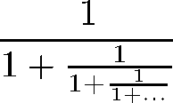
At first, this might seem hard to compute because the denominator never ends, just like the fraction itself. But that’s the trick: the denominator is equivalent to the fraction. Let’s call the answer x.

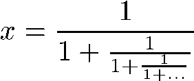
Since the denominator is also x, we can represent this fraction much more tractably:

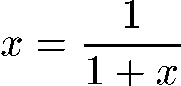
That’s equivalent to the familiar quadratic form:

The solution to this equation is approximately 0.618034, by the way. It’s the Golden Ratio—the ratio of successive Fibonacci numbers, believed by the Greeks to be the most pleasing ratio of height to width for architecture. The exact value of x is the square root of five, minus one, divided by two.

We can solve our equation using the familiar quadratic formula to find the largest root. However, suppose we only need the first three digits. From eyeballing the fraction, we know that x must be between 0 and 1; perhaps a for loop that begins at 0 and increases by .001 will find x faster. Here’s how we’d use the Benchmark module to verify that it won’t:

#!/usr/bin/perl

use Benchmark;

sub quadratic {     # Compute the larger root of a quadratic polynomial
    my ($a, $b, $c) = @_;
    return (-$b + sqrt($b*$b - 4*$a * $c)) / 2*$a;
}

sub bruteforce {    # Search linearly until we find a good-enough choice
    my ($low, $high) = @_;
    my $x;
    for ($x = $low; $x <= $high; $x += .001) {
        return $x if abs($x * ($x+1) - .999) < .001;
    }
}

timethese(10000, { quadratic  => 'quadratic(1, 1, -1)',
                   bruteforce => 'bruteforce(0, 1)'        });

After including the Benchmark module with use Benchmark, this program defines two subroutines. The first computes the larger root of any quadratic equation given its coefficients; the second iterates through a range of numbers looking for one that’s close enough. The Benchmark function timethese() is then invoked. The first argument, 10000, is the number of times to run each code snippet. The second argument is an anonymous hash with two key-value pairs. Each key-value pair maps your name for each code snippet (here, we’ve just used the names of the subroutines) to the snippet. After this line is reached, the following statistics are printed about a minute later (on our computer):

Benchmark: timing 10000 iterations of bruteforce, quadratic...
 bruteforce: 53 secs (12.07 usr  0.05 sys = 12.12 cpu)
  quadratic:  5 secs ( 1.17 usr  0.00 sys =  1.17 cpu)

This tells us that computing the quadratic formula isn’t just more elegant, it’s also 10 times faster, using only 1.17 CPU seconds compared to the for loop’s sluggish 12.12 CPU seconds.

Some tips for using the Benchmark module:

• Any test that takes less than one second is useless because startup latencies and caching complications will create misleading results. If a test takes less than one second, the Benchmark module might warn you:

  (warning: too few iterations for a reliable count)

  If your benchmarks execute too quickly, increase the number of repetitions.

• Be more interested in the CPU time (cpu = user + system, abbreviated usr and sys in the Benchmark module results) than in the first number, the real (wall clock) time spent. Measuring CPU time is more meaningful. In a multitasking operating system where multiple processes compete for the same CPU cycles, the time allocated to your process (the CPU time) will be less than the “wall clock” time (the 53 and 5 seconds in this example).

• If you’re testing a simple Perl expression, you might need to modify your code somewhat to benchmark it. Otherwise, Perl might evaluate your expression at compile time and report unrealistically high speeds as a result. (One sign of this optimization is the warning Useless use of ... in void context. That means that the operation doesn’t do anything, so Perl won’t bother executing it.) For a real-world example, see Chapter 6.

• The speed of your Perl program depends on just about everything: CPU clock speed, bus speed, cache size, amount of RAM, and your version of Perl.

Your mileage will vary.

Could you write a “meta-algorithm” that identifies the tradeoffs for your computer and chooses among several implementations accordingly? It might identify how long it takes to load your program (or the Perl interpreter) into memory, how long it takes to read or write data on disk, and so on. It would weigh the results and pick the fastest implementation for the problem. If you write this, let us know.

Floating-Point Numbers

Like most computer languages, Perl uses floating-point numbers for its calculations. You probably know what makes them different from integers—they have stuff after the decimal point. Computers can sometimes manipulate integers faster than floating-point numbers, so if your programs don’t need anything after the decimal point, you should place use integer at the top of your program:

#!/usr/bin/perl

use integer;     # Perform all arithmetic with integer-only operations.

$c = 7 / 3;      # $c is now 2

Keep in mind that floating-point numbers are not the same as the real numbers you learned about in math class. There are infinitely many real numbers between, say, 0 and 1, but Perl doesn’t have an infinite number of bits to store those real numbers. Corners must be cut.

Don’t believe us? In April 1997, someone submitted this to the perlbug mailing list:

Hi,

I'd appreciate if this is a known bug and if a patch is available.

int of (2.4/0.2) returns 11 instead of the expected 12.

It would seem that this poor fellow is correct: perl -e 'print int(2.4/0.2)' indeed prints 11. You might expect it to print 12, because two-point-four divided by oh-point-two is twelve, and the integer part of 12 is 12. Must be a bug in Perl, right?

Wrong. Floating-point numbers are not real numbers. When you divide 2.4 by 0.2, what you’re really doing is dividing Perl’s binary floating-point representation of 2.4 by Perl’s binary floating-point representation of 0.2. In all computer languages that use IEEE floating-point representations (not just Perl!) the result will be a smidgen less than 12, which is why int(2.4/0.2) is 11. Beware.

Temporary Variables

Suppose you want to convert an array of numbers from one logarithmic base to another. You’ll need the change of base law: . Perl provides the log function, which computes the natural (base ) logarithm, so we can use that. Question: are we better off storing in a variable and using that over and over again, or would be it better to compute it anew each time? Armed with the Benchmark module, we can find out:

#!/usr/bin/perl

use Benchmark;

sub logbase1 {                # Compute the value each time.
    my ($base, $numbers) = @_;
    my @result;
    for (my $i = 0; $i < @$numbers; $i++) {
        push @result, log ($numbers->[$i]) / log ($base);
    }
    return @result;
}

sub logbase2 {                # Store log $base in a temporary variable.
    my ($base, $numbers) = @_;
    my @result;
    my $logbase = log $base;
    for (my $i = 0; $i < @$numbers; $i++) {
        push @result, log ($numbers->[$i]) / $logbase;
    }
    return @result;
}

@numbers = (1..1000);

timethese (1000, { no_temp => 'logbase1( 10, \@numbers )',
                   temp => 'logbase2( 10, \@numbers )'  });

Here, we compute the logs of all the numbers between 1 and 1000. logbase1() and logbase2() are nearly identical, except that logbase2() stores the log of 10 in $logbase so that it doesn’t need to compute it each time. The result:

Benchmark: timing 1000 iterations of no_temp, temp...
      temp: 84 secs (63.77 usr  0.57 sys = 64.33 cpu)
   no_temp: 98 secs (84.92 usr  0.42 sys = 85.33 cpu)

The temporary variable results in a 25% speed increase—on my machine and with my particular Perl configuration. But temporary variables aren’t always efficient; consider two nearly identical subroutines that compute the volume of an n-dimensional sphere. The formula is . Computing the factorial of a fractional integer is a little tricky and requires some extra code—the if ($n % 2) block in both subroutines that follow. (For more about factorials, see Section 11.1.5 in Chapter 11.) The volume_var() subroutine assigns to a temporary variable, $denom; the volume_novar() subroutine returns the result directly.

use constant pi => 3.14159265358979;

sub volume_var {
    my ($r, $n) = @_;
    my $denom;
    if ($n % 2) {
        $denom = sqrt(pi) * factorial(2 * (int($n / 2)) + 2) /
            factorial(int($n / 2) + 1) / (4 ** (int($n / 2) + 1));
    } else {
        $denom = factorial($n / 2);
    }
    return ($r ** $n) * (pi ** ($n / 2)) / $denom;
}

sub volume_novar {
    my ($r, $n) = @_;
    if ($n % 2) {
        return ($r ** $n) * (pi ** ($n / 2)) /
        (sqrt(pi) * factorial(2 * (int($n / 2)) + 2) /
         factorial(int($n / 2) + 1) / (4 ** (int($n / 2) + 1)));
    } else {
        return ($r ** $n) * (pi ** ($n / 2)) / factorial($n / 2);
    }
}

The results:

volume_novar: 58 secs (29.62 usr  0.00 sys = 29.62 cpu)
  volume_var: 64 secs (31.87 usr  0.02 sys = 31.88 cpu)

Here, the temporary variable $denom slows down the code instead: 7.6% on the same computer that saw the 25% speed increase earlier. A second computer showed a larger decrease in speed: a 10% speed increase for changing bases, and a 12% slowdown for computing hypervolumes. Your results will be different.

Caching

Storing something in a temporary variable is a specific example of a general technique: caching. It means simply that data likely to be used in the future is kept “nearby.” Caching is used by your computer’s CPU, by your web browser, and by your brain; for instance, when you visit a web page, your web browser stores it on a local disk. That way, when you visit the page again, it doesn’t have to ferry the data over the Internet.

One caching principle that’s easy to build into your program is never compute the same thing twice. Save results in variables while your program is running, or on disk when it’s not. There’s even a CPAN module that optimizes subroutines in just this way: Memoize.pm. Here’s an example:

use Memoize;
memoize 'binary_search';     # Turn on caching for binary_search()

binary_search("wolverine");  # This executes normally...
binary_search("wolverine");  # ...but this returns immediately

The memoize 'binary_search'; line turns binary_search() (which we defined earlier) into a memoizing subroutine. Whenever you invoke binary_search() with a particular argument, it remembers the result. If you call it with that same argument later, it will use the stored result and return immediately instead of performing the binary search all over again.

You can find a nonmemoizing example of caching in Section 12.2.1 in Chapter 12.

Evaluating Algorithms: O(N) Notation

The Benchmark module shown earlier tells you the speed of your program, not the speed of your algorithm. Remember our two approaches for searching through a list of words: proceeding through the entire list (dictionary) sequentially, and binary search. Obviously, binary search is more efficient, but how can we speak about efficiency if everything depends on the implementation?

In computer science, the speed (and occasionally, the space) of an algorithm is expressed with a mathematical symbolism informally referred to as O(N) notation. typically refers to the number of data items to be processed, although it might be some other quantity. If an algorithm runs in time, then it has order of growth —the number of operations is proportional to the logarithm of the number of elements fed to the algorithm. If you triple the number of elements, the algorithm will require approximately log3 more operations, give or take a constant multiplier. Binary search is an algorithm. If we double the size of the list of words, the effect is insignificant—a single extra iteration through the while loop.

In contrast, our linear search that cycles through the word list item by item is an algorithm. If we double the size of the list, the number of operations doubles. Of course, the incremental search won’t always take longer than the binary search; if the target word occurs near the very beginning of the alphabet, the linear search will be faster. The order of growth is a statement about the overall behavior of the algorithm; individual runs will vary.

Furthermore, the notation (and similar notations we’ll see shortly) measure the asymptotic behavior of an algorithm. What we care about is not how long the algorithm takes for a input of a certain size, merely how it changes as the input grows without bound. The difference is subtle but important.

notation is often used casually to mean the empirical running time of an algorithm. In the formal study of algorithms, there are five “proper” measurements of running time, shown in Table 1-3.

Table 1-3. Classes of Orders of Growth

Function	Meaning
	“The algorithm won’t take longer than "
	“The algorithm won’t take longer than , give or take a constant multiplier”
	“The algorithm will take as long as , give or take a constant multiplier”
	“The algorithm will take longer than , give or take a constant multiplier”
	“The algorithm will take longer than "

If we say that an algorithm is , we mean that its best-case running time is proportional to the square of the number of inputs, give or take a constant multiplier.

These are simplified descriptions; for more rigorous definitions, see Introduction to Algorithms, published by MIT Press. For instance, our binary search algorithm is and , but it’s also —any algorithm is also because, asymptotically, is less than . However, it’s not , because isn’t an asymptotically tight bound for .

These notations are sometimes used to describe the average-case or the best-case behavior, but only rarely. Best-case analysis is usually pointless, and average-case analysis is typically difficult. The famous counterexample to this is quicksort, one of the most popular algorithms for sorting a collection of elements. Quicksort is worst case and average case. You’ll learn about quicksort in Chapter 4.

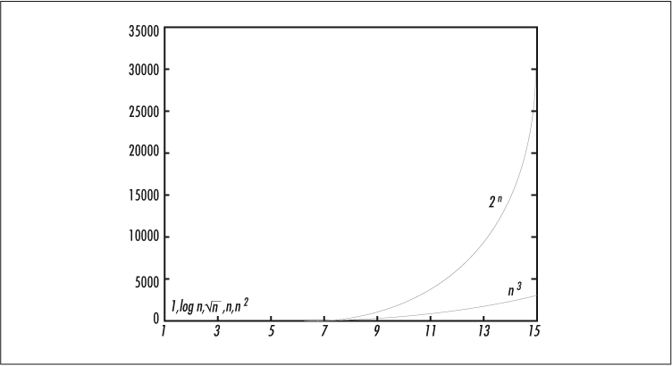
In case this all seems pedantic, consider how growth functions compare. Table 1-4 lists eight growth functions and their values given a million data points.

Table 1-4. An Order of Growth Sampler

Growth Function	Value for N = 1,000,000
	1
	13.8
	1000
	1,000,000
N log N	13,815,510
	1,000,000,000,000
	1,000,000,000,000,000,000
	A number with 693,148 digits.

Figure 1-1 shows how these functions compare when N varies from 1 to 2.

Figure 1-1. Orders of growth between 1 and 2

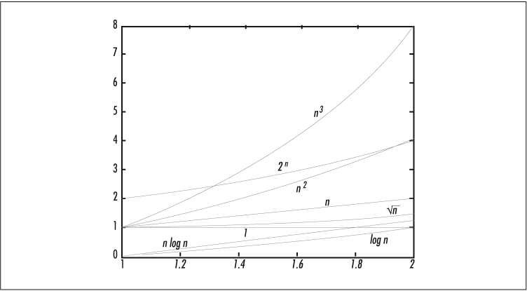
In Figure 1-1, all these orders of growth seem comparable. But see how they diverge as we extend N to 15 in Figure 1-2.

Figure 1-2. Orders of growth between 1 and 15

If you consider sorting records, you’ll see why the choice of algorithm is important.

Don’t cheat

We had to jump through some hoops when we modified our binary search to work with a newline-delimited list of words in a file. We could have simplified the code somewhat if our program had scanned through the file first, identifying where the newlines are. Then we wouldn’t have to worry about moving around in the file and ending up in the middle of a word—we’d redefine our window so that it referred to lines instead of bytes. Our program would be smaller and possibly even faster (but not likely).

That’s cheating. Even though this initialization step is performed before entering the binary_search() subroutine, it still needs to go through the file line by line, and since there are as many lines as words, our implementation is now only instead of the much more desirable . The difference might only be a fraction of a second for a few hundred thousand words, but the cardinal rule battered into every computer scientist is that we should always design for scalability. The program used for a quarter-million words today might be called upon for a quarter-trillion words tomorrow.

Recurrent Themes in Algorithms

Each algorithm in this book is a strategy—a particular trick for solving some problem. The remainder of this chapter looks at three intertwined ideas, recursion, divide and conquer, and dynamic programming, and concludes with an observation about representing data.

Recursion

re·cur·sion \ri-'ker-zhen\ n See RECURSION

Something that is defined in terms of itself is said to be recursive. A function that calls itself is recursive; so is an algorithm defined in terms of itself. Recursion is a fundamental concept in computer science; it enables elegant solutions to certain problems. Consider the task of computing the factorial of , denoted and defined as the product of all the numbers from 1 to . You could define a factorial() subroutine without recursion:

# factorial($n) computes the factorial of $n,
#   using an iterative algorithm.
sub factorial {
    my ($n) = shift;
    my ($result, $i) = (1, 2);
    for ( ; $i <= $n; $i++) {
        $result *= $i;
    }
    return $result;
}

It’s much cleaner to use recursion:

# factorial_recursive($n) computes the factorial of $n,
#   using a recursive algorithm.
sub factorial_recursive {
    my ($n) = shift;
    return $n if $n <= 2;
    return $n * factorial_recursive($n - 1);
}

Both of these subroutines are , since computing the factorial of requires multiplications. The recursive implementation is cleaner, and you might suspect faster. However, it takes four times as long on our computers, because there’s overhead involved whenever you call a subroutine. The nonrecursive (or iterative) subroutine just amasses the factorial in an integer, while the recursive subroutine has to invoke itself repeatedly—and subroutine invocations take a lot of time.

As it turns out, there is an algorithm to approximate the factorial. That speed comes at a price: it’s not exact.

sub factorial_approx {
    return sqrt (1.5707963267949 * $_[0]) *
        (($_[0] / 2.71828182845905) ** $_[0]);
}

We could have implemented binary search recursively also, with binary_search() accepting $low and $high as arguments, checking the current word, adjusting $low and $high, and calling itself with the new window. The slowdown would have been comparable.

Many interesting algorithms are best conveyed as recursions and often most easily implemented that way as well. However, recursion is never necessary: any algorithm that can be expressed recursively can also be written iteratively. Some compilers are able to convert a particular class of recursion called tail recursion into iteration, with the corresponding increase in speed. Perl’s compiler can’t. Yet.

Divide and Conquer

Many algorithms use a strategy called divide and conquer to make problems tractable. Divide and conquer means that you break a tough problem into smaller, more solvable subproblems, solve them, and then combine their solutions to “conquer” the original problem.^[3]

Divide and conquer is nothing more than a particular flavor of recursion. Consider the mergesort algorithm, which you’ll learn about in Chapter 4. It sorts a list of items by immediately breaking the list in half and mergesorting each half. Thus, the list is divided into halves, quarters, eighths, and so on, until “little” invocations of mergesort are fed a simple pair of numbers. These are conquered—that is, compared—and then the newly sorted sublists are merged into progressively larger sorted lists, culminating in a complete sort of the original list.

Dynamic Programming

Dynamic programming is sometimes used to describe any algorithm that caches its intermediate results so that it never needs to compute the same subproblem twice. Memoizing is an example of this sense of dynamic programming.

There is another, broader definition of dynamic programming. The divide-and-conquer strategy discussed in the last section is top-down: you take a big problem and break it into smaller, independent subproblems. When the subproblems depend on each other, you may need to think about the solution from the bottom up: solving more subproblems than you need to, and after some thought, deciding how to combine them. In other words, your algorithm performs a little pregame analysis—examining the data in order to deduce how best to proceed. Thus, it’s “dynamic” in the sense that the algorithm doesn’t know how it will tackle the data until after it starts. In the matrix chain problem, described in Chapter 7, a set of matrices must be multiplied together. The number of individual (scalar) multiplications varies widely depending on the order in which you multiply the matrices, so the algorithm simply computes the optimal order beforehand.

Choosing the Right Representation

The study of algorithms is lofty and academic—a subset of computer science concerned with mathematical elegance, abstract tricks, and the refinement of ingenious strategies developed over decades. The perspective suggested in many algorithms textbooks and university courses is that an algorithm is like a magic incantation, a spell created by a wizardly sage and passed down through us humble chroniclers to you, the willing apprentice.

However, the dirty truth is that algorithms get more credit than they deserve. The metaphor of an algorithm as a spell or battle strategy falls flat on close inspection; the most important problem-solving ability is the capacity to reformulate the problem—to choose an alternative representation that facilitates a solution. You can look at logarithms this way: by replacing numbers with their logarithms, you turn a multiplication problem into an addition problem. (That’s how slide rules work.) Or, by representing shapes in terms of angle and radius instead of by the more familiar Cartesian coordinates, it becomes easy to represent a circle (but hard to represent a square).

Data structures—the representations for your data—don’t have the status of algorithms. They aren’t typically named after their inventors; the phrase “well-designed” is far more likely to precede “algorithm” than “data structure.” Nevertheless, they are just as important as the algorithms themselves, and any book about algorithms must discuss how to design, choose, and use data structures. That’s the subject of the next two chapters.

---

^[1] Precedes in ASCII order, not dictionary order! See Section 4.1.2 in Chapter 4.

^[2] We won’t consider “design efficiency”—how long it takes the programmer to create the program. But the fastest program in the world is no good if it was due three weeks ago. You can sometimes write faster programs in C, but you can always write programs faster in Perl.

^[3] The tactic should more properly be called divide, conquer, and combine, but that weakens the programmer-as-warrior militaristic metaphor somewhat.