Natural Language Processing with PyTorch

Chapter 4. Feed-Forward Networks for Natural Language Processing

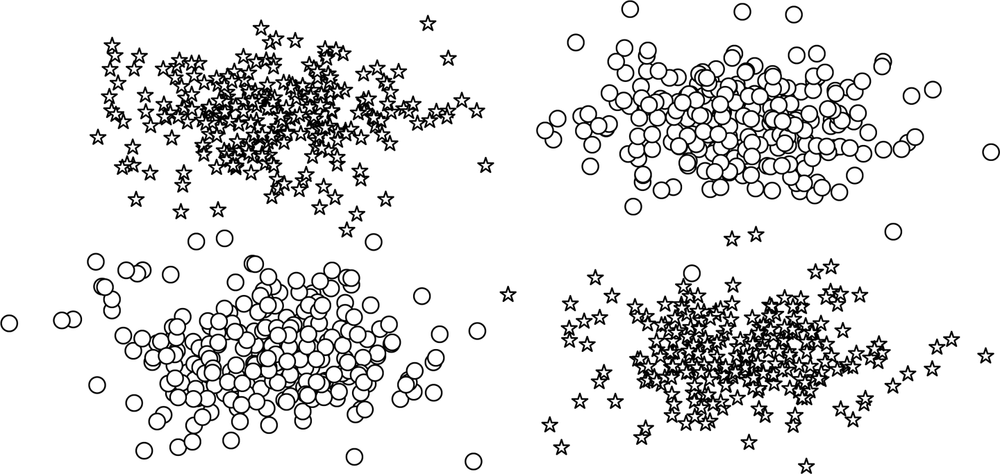
In Chapter 3, we covered the foundations of neural networks by looking at the perceptron, the simplest neural network that can exist. One of the historic downfalls of the perceptron was that it cannot learn modestly nontrivial patterns present in data. For example, take a look at the plotted data points in Figure 4-1. This is equivalent to an either-or (XOR) situation in which the decision boundary cannot be a single straight line (otherwise known as being linearly separable). In this case, the perceptron fails.

Figure 4-1. Two classes in the XOR dataset plotted as circles and stars. Notice how no single line can separate the two classes.

In this chapter, we explore a family of neural network models traditionally called feed-forward networks. We focus on two kinds of feed-forward neural networks: the multilayer perceptron (MLP) and the convolutional neural network (CNN).¹ The multilayer perceptron structurally extends the simpler perceptron we studied in Chapter 3 by grouping many perceptrons in a single layer and stacking multiple layers together. We cover multilayer perceptrons in just a moment and show their use in multiclass classification in “Example: Surname Classification with an MLP”.

The second kind of feed-forward neural networks studied in this chapter, the convolutional neural network, is deeply inspired by windowed filters in the processing of digital signals. Through this windowing property, CNNs are able to learn localized patterns in their inputs, which has not only made them the workhorse of computer vision but also an ideal candidate for detecting substructures in sequential data, such as words and sentences. We explore CNNs in “Convolutional Neural Networks” and demonstrate their use in “Example: Classifying Surnames by Using a CNN”.

In this chapter, MLPs and CNNs are grouped together because they are both feed-forward neural networks and stand in contrast to a different family of neural networks, recurrent neural networks (RNNs), which allow for feedback (or cycles) such that each computation is informed by the previous computation. In Figures 6 and 7, we cover RNNs and why it can be beneficial to allow cycles in the network structure.

As we walk through these different models, one useful way to make sure you understand how things work is to pay attention to the size and shape of the data tensors as they are being computed. Each type of neural network layer has a specific effect on the size and shape of the data tensor it is computing on, and understanding that effect can be extremely conducive to a deeper understanding of these models.

The Multilayer Perceptron

The multilayer perceptron is considered one of the most basic neural network building blocks. The simplest MLP is an extension to the perceptron of Chapter 3. The perceptron takes the data vector² as input and computes a single output value. In an MLP, many perceptrons are grouped so that the output of a single layer is a new vector instead of a single output value. In PyTorch, as you will see later, this is done simply by setting the number of output features in the Linear layer. An additional aspect of an MLP is that it combines multiple layers with a nonlinearity in between each layer.

The simplest MLP, displayed in Figure 4-2, is composed of three stages of representation and two Linear layers. The first stage is the input vector. This is the vector that is given to the model. In “Example: Classifying Sentiment of Restaurant Reviews”, the input vector was a collapsed one-hot representation of a Yelp review. Given the input vector, the first Linear layer computes a hidden vector—the second stage of representation. The hidden vector is called such because it is the output of a layer that’s between the input and the output. What do we mean by “output of a layer”? One way to understand this is that the values in the hidden vector are the output of different perceptrons that make up that layer. Using this hidden vector, the second Linear layer computes an output vector. In a binary task like classifying the sentiment of Yelp reviews, the output vector could still be of size 1. In a multiclass setting, as you’ll see in “Example: Surname Classification with an MLP”, the size of the output vector is equal to the number of classes. Although in this illustration we show only one hidden vector, it is possible to have multiple intermediate stages, each producing its own hidden vector. Always, the final hidden vector is mapped to the output vector using a combination of Linear layer and a nonlinearity.

Figure 4-2. A visual representation of an MLP with two linear layers and three stages of representation—the input vector, the hidden vector, and the output vector.

The power of MLPs comes from adding the second Linear layer and allowing the model to learn an intermediate representation that is linearly separable—a property of representations in which a single straight line (or more generally, a hyperplane) can be used to distinguish the data points by which side of the line (or hyperplane) they fall on. Learning intermediate representations that have specific properties, like being linearly separable for a classification task, is one of the most profound consequences of using neural networks and is quintessential to their modeling capabilities. In the next section, we take a much closer, in-depth look at what that means.

A Simple Example: XOR

Let’s take a look at the XOR example described earlier and see what would happen with a perceptron versus an MLP. In this example, we train both the perceptron and an MLP in a binary classification task: identifying stars and circles. Each data point is a 2D coordinate. Without diving into the implementation details yet, the final model predictions are shown in Figure 4-3. In this plot, incorrectly classified data points are filled in with black, whereas correctly classified data points are not filled in. In the left panel, you can see that the perceptron has difficulty in learning a decision boundary that can separate the stars and circles, as evidenced by the filled in shapes. However, the MLP (right panel) learns a decision boundary that classifies the stars and circles much more accurately.

Figure 4-3. The learned solutions from the perceptron (left) and MLP (right) for the XOR problem. The true class of each data point is the point’s shape: star or circle. Incorrect classifications are filled in with black and correct classifications are not filled in. The lines are the decision boundaries of each model. In the left panel, a perceptron learns a decision boundary that cannot correctly separate the circles from the stars. In fact, no single line can. In the right panel, an MLP has learned to separate the stars from the circles.

Although it appears in the plot that the MLP has two decision boundaries, and that is its advantage, it is actually just one decision boundary! The decision boundary just appears that way because the intermediate representation has morphed the space to allow one hyperplane to appear in both of those positions. In Figure 4-4, we can see the intermediate values being computed by the MLP. The shapes of the points indicate the class (star or circle). What we see is that the neural network (an MLP in this case) has learned to “warp” the space in which the data lives so that it can divide the dataset with a single line by the time it passes through the final layer.

Figure 4-4. The input and intermediate representations for an MLP. From left to right: (1) the input to the network, (2) the output of the first linear module, (3) the output of the first nonlinearity, and (4) the output of the second linear module. As you can see, the output of the first linear module groups the circles and stars, whereas the output of the second linear module reorganizes the data points to be linearly separable.

In contrast, as Figure 4-5 demonstrates, the perceptron does not have an extra layer that lets it massage the shape of the data until it becomes linearly separable.

Figure 4-5. The input and output representations of the perceptron. Because it does not have an intermediate representation to group and reorganize as the MLP can, it cannot separate the circles and stars.

Implementing MLPs in PyTorch

In the previous section, we outlined the core ideas of the MLP. In this section, we walk through an implementation in PyTorch. As described, the MLP has an additional layer of computation beyond the simpler perceptron we saw in Chapter 3. In the implementation that we present in Example 4-1, we instantiate this idea with two of PyTorch’s Linear modules. The Linear objects are named fc1 and fc2, following a common convention that refers to a Linear module as a “fully connected layer,” or “fc layer” for short.³ In addition to these two Linear layers, there is a Rectified Linear Unit (ReLU) nonlinearity (introduced in Chapter 3, in “Activation Functions”) which is applied to the output of the first Linear layer before it is provided as input to the second Linear layer. Because of the sequential nature of the layers, you must take care to ensure that the number of outputs in a layer is equal to the number of inputs to the next layer. Using a nonlinearity between two Linear layers is essential because without it, two Linear layers in sequence are mathematically equivalent to a single Linear layer⁴ and thus unable to model complex patterns. Our implementation of the MLP implements only the forward pass of the backpropagation. This is because PyTorch automatically figures out how to do the backward pass and gradient updates based on the definition of the model and the implementation of the forward pass.

Example 4-1. Multilayer perceptron using PyTorch

import torch.nn as nn
import torch.nn.functional as F

class MultilayerPerceptron(nn.Module):
    def __init__(self, input_dim, hidden_dim, output_dim):
        """
        Args:
            input_dim (int): the size of the input vectors
            hidden_dim (int): the output size of the first Linear layer
            output_dim (int): the output size of the second Linear layer
        """
        super(MultilayerPerceptron, self).__init__()
        self.fc1 = nn.Linear(input_dim, hidden_dim)
        self.fc2 = nn.Linear(hidden_dim, output_dim)

    def forward(self, x_in, apply_softmax=False):
        """The forward pass of the MLP
        
        Args:
            x_in (torch.Tensor): an input data tensor 
                x_in.shape should be (batch, input_dim)
            apply_softmax (bool): a flag for the softmax activation
                should be false if used with the cross-entropy losses
        Returns:
            the resulting tensor. tensor.shape should be (batch, output_dim)
        """
        intermediate = F.relu(self.fc1(x_in))
        output = self.fc2(intermediate)
        
        if apply_softmax:
            output = F.softmax(output, dim=1).
        return output

In Example 4-2, we instantiate the MLP. Due to the generality of the MLP implementation, we can model inputs of any size. To demonstrate, we use an input dimension of size 3, an output dimension of size 4, and a hidden dimension of size 100. Notice how in the output of the print statement, the number of units in each layer nicely line up to produce an output of dimension 4 for an input of dimension 3.

Example 4-2. An example instantiation of an MLP

Input[0]	batch_size = 2 # number of samples input at once input_dim = 3 hidden_dim = 100 output_dim = 4 # Initialize model mlp = MultilayerPerceptron(input_dim, hidden_dim, output_dim) print(mlp)
Output[0]	MultilayerPerceptron( (fc1): Linear(in_features=3, out_features=100, bias=True) (fc2): Linear(in_features=100, out_features=4, bias=True) (relu): ReLU() )

We can quickly test the “wiring” of the model by passing some random inputs, as shown in Example 4-3. Because the model is not yet trained, the outputs are random. Doing this is a useful sanity check before spending time training a model. Notice how PyTorch’s interactivity allows us to do all this in real time during development, in a way not much different from using NumPy or Pandas.

Example 4-3. Testing the MLP with random inputs

Input[0]	def describe(x): print("Type: {}".format(x.type())) print("Shape/size: {}".format(x.shape)) print("Values: \n{}".format(x)) x_input = torch.rand(batch_size, input_dim) describe(x_input)
Output[0]	Type: torch.FloatTensor Shape/size: torch.Size([2, 3]) Values: tensor([[ 0.8329, 0.4277, 0.4363], [ 0.9686, 0.6316, 0.8494]])
Input[1]	y_output = mlp(x_input, apply_softmax=False) describe(y_output)
Output[1]	Type: torch.FloatTensor Shape/size: torch.Size([2, 4]) Values: tensor([[-0.2456, 0.0723, 0.1589, -0.3294], [-0.3497, 0.0828, 0.3391, -0.4271]])

It is important to learn how to read inputs and outputs of PyTorch models. In the preceding example, the output of the MLP model is a tensor that has two rows and four columns. The rows in this tensor correspond to the batch dimension, which is the number of data points in the minibatch. The columns are the final feature vectors for each data point.⁵ In some cases, such as in a classification setting, the feature vector is a prediction vector. The name “prediction vector” means that it corresponds to a probability distribution. What happens with the prediction vector depends on whether we are currently conducting training or performing inference. During training, the outputs are used as is with a loss function and a representation of the target class labels.⁶ We cover this in depth in “Example: Surname Classification with an MLP”.

However, if you want to turn the prediction vector into probabilities, an extra step is required. Specifically, you require the softmax activation function, which is used to transform a vector of values into probabilities. The softmax function has many roots. In physics, it is known as the Boltzmann or Gibbs distribution; in statistics, it’s multinomial logistic regression; and in the natural language processing (NLP) community it’s known as the maximum entropy (MaxEnt) classifier.⁷ Whatever the name, the intuition underlying the function is that large positive values will result in higher probabilities, and lower negative values will result in smaller probabilities. In Example 4-3, the apply_softmax argument applies this extra step. In Example 4-4, you can see the same output, but this time with the apply_softmax flag set to True.

Example 4-4. Producing probabilistic outputs with a multilayer perceptron classifier (notice the apply_softmax = True option)

Input[0]	y_output = mlp(x_input, apply_softmax=True) describe(y_output)
Output[0]	Type: torch.FloatTensor Shape/size: torch.Size([2, 4]) Values: tensor([[ 0.2087, 0.2868, 0.3127, 0.1919], [ 0.1832, 0.2824, 0.3649, 0.1696]])

To conclude, MLPs are stacked Linear layers that map tensors to other tensors. Nonlinearities are used between each pair of Linear layers to break the linear relationship and allow for the model to twist the vector space around. In a classification setting, this twisting should result in linear separability between classes. Additionally, you can use the softmax function to interpret MLP outputs as probabilities, but you should not use softmax with specific loss functions,⁸ because the underlying implementations can leverage superior mathematical/computational shortcuts.

Example: Surname Classification with an MLP

In this section, we apply the MLP to the task of classifying surnames to their country of origin. Inferring demographic information (like nationality) from publicly observable data has applications from product recommendations to ensuring fair outcomes for users across different demographics. However, demographic and other self-identifying attributes are collectively called “protected attributes.” You must exercise care in the use of such attributes in modeling and in products.⁹ We begin by splitting the characters of each surname and treating them the same way we treated words in “Example: Classifying Sentiment of Restaurant Reviews”. Aside from the data difference, character-level models are mostly similar to word-based models in structure and implementation.¹⁰

An important lesson that you should take away from this example is that implementation and training of an MLP is a straightforward progression from the implementation and training we saw for a perceptron in Chapter 3. In fact, we point back to the example in Chapter 3 throughout the book as the place to go to get a more thorough overview of these components. Further, we will not include code that you can see in “Example: Classifying Sentiment of Restaurant Reviews” If you want to see the example code in one place, we highly encourage you to follow along with the supplementary material.¹¹

This section begins with a description of the surnames dataset and its preprocessing steps. Then, we step through the pipeline from a surname string to a vectorized minibatch using the Vocabulary, Vectorizer, and DataLoader classes. If you read through Chapter 3, you should recognize these auxiliary classes as old friends, with some small modifications.

We continue the section by describing the surnameclassifier model and the thought process underlying its design. The MLP is similar to the perceptron example we saw in Chapter 3, but in addition to the model change, we introduce multiclass outputs and their corresponding loss functions in this example. After describing the model, we walk through the training routine. This is quite similar to what you saw in “The Training Routine” so for brevity we do not go into as much depth here as we did in that section. We strongly recommend that you refer back that section for additional clarification.

We conclude the example by evaluating the model on the test portion of the dataset and describing the inference procedure on a new surname. A nice property of multiclass predictions is that we can look at more than just the top prediction, and we additionally walk through how to infer the top k predictions for a new surname.

The Surnames Dataset

In this example, we introduce the surnames dataset, a collection of 10,000 surnames from 18 different nationalities collected by the authors from different name sources on the internet. This dataset will be reused in several examples in the book and has several properties that make it interesting. The first property is that it is fairly imbalanced. The top three classes account for more than 60% of the data: 27% are English, 21% are Russian, and 14% are Arabic. The remaining 15 nationalities have decreasing frequency—a property that is endemic to language, as well. The second property is that there is a valid and intuitive relationship between nationality of origin and surname orthography (spelling). There are spelling variations that are strongly tied to nation of origin (such in “O’Neill,” “Antonopoulos,” “Nagasawa,” or “Zhu”).

To create the final dataset, we began with a less-processed version than what is included in this book’s supplementary material and performed several dataset modification operations. The first was to reduce the imbalance—the original dataset was more than 70% Russian, perhaps due to a sampling bias or a proliferation in unique Russian surnames. For this, we subsampled this overrepresented class by selecting a randomized subset of surnames labeled as Russian. Next, we grouped the dataset based on nationality and split the dataset into three sections: 70% to a training dataset, 15% to a validation dataset, and the last 15% to the testing dataset, such that the class label distributions are comparable across the splits.

The implementation of the SurnameDataset is nearly identical to the ReviewDataset as seen in “Example: Classifying Sentiment of Restaurant Reviews”, with only minor differences in how the __getitem__() method is implemented.¹² Recall that the dataset classes presented in this book inherit from PyTorch’s Dataset class, and as such, we need to implement two functions: the __getitem__() method, which returns a data point when given an index; and the __len__() method, which returns the length of the dataset. The difference between the example in Chapter 3 and this example is in the __getitem__ method as shown in Example 4-5. Rather than returning a vectorized review as in “Example: Classifying Sentiment of Restaurant Reviews”, it returns a vectorized surname and the index corresponding to its nationality.

Example 4-5. Implementing SurnameDataset.__getitem__()

class SurnameDataset(Dataset):
    # Implementation is nearly identical to Example 3-14

    def __getitem__(self, index):
        row = self._target_df.iloc[index]
        surname_vector = \
            self._vectorizer.vectorize(row.surname)
        nationality_index = \
            self._vectorizer.nationality_vocab.lookup_token(row.nationality)

        return {'x_surname': surname_vector,
                'y_nationality': nationality_index}

Vocabulary, Vectorizer, and DataLoader

To classify surnames using their characters, we use the Vocabulary, Vectorizer, and DataLoader to transform surname strings into vectorized minibatches. These are the same data structures used in “Example: Classifying Sentiment of Restaurant Reviews”, exemplifying a polymorphism that treats the character tokens of surnames in the same way as the word tokens of Yelp reviews. Instead of vectorizing by mapping word tokens to integers, the data is vectorized by mapping characters to integers.

The Vocabulary class

The Vocabulary class used in this example is exactly the same as the one used in Example 3-16 to map the words in Yelp reviews to their corresponding integers. As a brief overview, the Vocabulary is a coordination of two Python dictionaries that form a bijection between tokens (characters, in this example) and integers; that is, the first dictionary maps characters to integer indices, and the second maps the integer indices to characters. The add_token() method is used to add new tokens into the Vocabulary, the lookup_token() method is used to retrieve an index, and the lookup_index() method is used to retrieve a token given an index (which is useful in the inference stage). In contrast with the Vocabulary for Yelp reviews, we use a one-hot representation¹³ and do not count the frequency of characters and restrict only to frequent items. This is mainly because the dataset is small and most characters are frequent enough.

The SurnameVectorizer

Whereas the Vocabulary converts individual tokens (characters) to integers, the SurnameVectorizer is responsible for applying the Vocabulary and converting a surname into a vector. The instantiation and use are very similar to the ReviewVectorizer in “Vectorizer”, but with one key difference: the string is not split on whitespace. Surnames are sequences of characters, and each character is an individual token in our Vocabulary. However, until “Convolutional Neural Networks”, we will ignore the sequence information and create a collapsed one-hot vector representation of the input by iterating over each character in the string input. We designate a special token, UNK, for characters not encountered before. The UNK symbol is still used in the character Vocabulary because we instantiate the Vocabulary from the training data only and there could be unique characters in the validation or testing data.¹⁴

You should note that although we used the collapsed one-hot representation in this example, you will learn about other methods of vectorization in later chapters that are alternatives to, and sometimes better than, the one-hot encoding. Specifically, in “Example: Classifying Surnames by Using a CNN”, you will see a one-hot matrix in which each character is a position in the matrix and has its own one-hot vector. Then, in Chapter 5, you will learn about the embedding layer, the vectorization that returns a vector of integers, and how those are used to create a matrix of dense vectors. But for now, let’s take a look at the code for the SurnameVectorizer in Example 4-6.

Example 4-6. Implementing SurnameVectorizer

class SurnameVectorizer(object):
    """ The Vectorizer which coordinates the Vocabularies and puts them to use"""
    def __init__(self, surname_vocab, nationality_vocab):
        self.surname_vocab = surname_vocab
        self.nationality_vocab = nationality_vocab

    def vectorize(self, surname):
        """Vectorize the provided surname

        Args:
            surname (str): the surname
        Returns:
            one_hot (np.ndarray): a collapsed one-hot encoding
        """
        vocab = self.surname_vocab
        one_hot = np.zeros(len(vocab), dtype=np.float32)
        for token in surname:
            one_hot[vocab.lookup_token(token)] = 1
        return one_hot

    @classmethod
    def from_dataframe(cls, surname_df):
        """Instantiate the vectorizer from the dataset dataframe
        
        Args:
            surname_df (pandas.DataFrame): the surnames dataset
        Returns:
            an instance of the SurnameVectorizer
        """
        surname_vocab = Vocabulary(unk_token="@")
        nationality_vocab = Vocabulary(add_unk=False)

        for index, row in surname_df.iterrows():
            for letter in row.surname:
                surname_vocab.add_token(letter)
            nationality_vocab.add_token(row.nationality)

        return cls(surname_vocab, nationality_vocab)

The SurnameClassifier Model

The SurnameClassifier (Example 4-7) is an implementation of the MLP introduced earlier in this chapter. The first Linear layer maps the input vectors to an intermediate vector, and a nonlinearity is applied to that vector. A second Linear layer maps the intermediate vector to the prediction vector.

In the last step, the softmax function is optionally applied to make sure the outputs sum to 1; that is, are interpreted as “probabilities.”¹⁵ The reason it is optional has to do with the mathematical formulation of the loss function we use—the cross-entropy loss, introduced in “Loss Functions”. Recall that cross-entropy loss is most desirable for multiclass classification, but computation of the softmax during training is not only wasteful but also not numerically stable in many situations.

Example 4-7. The SurnameClassifier using an MLP

import torch.nn as nn
import torch.nn.functional as F

class SurnameClassifier(nn.Module):
    """ A 2-layer multilayer perceptron for classifying surnames """
    def __init__(self, input_dim, hidden_dim, output_dim):
        """
        Args:
            input_dim (int): the size of the input vectors
            hidden_dim (int): the output size of the first Linear layer
            output_dim (int): the output size of the second Linear layer
        """
        super(SurnameClassifier, self).__init__()
        self.fc1 = nn.Linear(input_dim, hidden_dim)
        self.fc2 = nn.Linear(hidden_dim, output_dim)

    def forward(self, x_in, apply_softmax=False):
        """The forward pass of the classifier
        
        Args:
            x_in (torch.Tensor): an input data tensor 
                x_in.shape should be (batch, input_dim)
            apply_softmax (bool): a flag for the softmax activation
                should be false if used with the cross-entropy losses
        Returns:
            the resulting tensor. tensor.shape should be (batch, output_dim).
        """
        intermediate_vector = F.relu(self.fc1(x_in))
        prediction_vector = self.fc2(intermediate_vector)

        if apply_softmax:
            prediction_vector = F.softmax(prediction_vector, dim=1)

        return prediction_vector

The Training Routine

Although we use a different model, dataset, and loss function in this example, the training routine remains the same as that described in the previous chapter. Thus, in Example 4-8, we show only the args and the major differences between the training routine in this example and the one in “Example: Classifying Sentiment of Restaurant Reviews”.

Example 4-8. Hyperparameters and program options for the MLP-based Yelp review classifier

args = Namespace(
    # Data and path information
    surname_csv="data/surnames/surnames_with_splits.csv",
    vectorizer_file="vectorizer.json",
    model_state_file="model.pth",
    save_dir="model_storage/ch4/surname_mlp",
    # Model hyper parameters
    hidden_dim=300
    # Training  hyper parameters
    seed=1337,
    num_epochs=100,
    early_stopping_criteria=5,
    learning_rate=0.001,
    batch_size=64,
    # Runtime options omitted for space
)

The most notable difference in training has to do with the kinds of outputs in the model and the loss function being used. In this example, the output is a multiclass prediction vector that can be turned into probabilities. The loss functions that can be used for this output are limited to CrossEntropyLoss() and NLLLoss(). Due to its simplifications, we use CrossEntropyLoss().

In Example 4-9, we show the instantiations for the dataset, the model, the loss function, and the optimizer. These instantiations should look nearly identical to those from the example in Chapter 3. In fact, this pattern will repeat for every example in later chapters in this book.

Example 4-9. Instantiating the dataset, model, loss, and optimizer

dataset = SurnameDataset.load_dataset_and_make_vectorizer(args.surname_csv)
vectorizer = dataset.get_vectorizer()

classifier = SurnameClassifier(input_dim=len(vectorizer.surname_vocab), 
                               hidden_dim=args.hidden_dim, 
                               output_dim=len(vectorizer.nationality_vocab))

classifier = classifier.to(args.device)    

loss_func = nn.CrossEntropyLoss(dataset.class_weights)
optimizer = optim.Adam(classifier.parameters(), lr=args.learning_rate)

The training loop

The training loop for this example is nearly identical to that described in compared to the training loop in “The training loop”, except for the variable names. Specifically, Example 4-10 shows that different keys are used to get the data out of the batch_dict. Aside from this cosmetic difference, the functionality of the training loop remains the same. Using the training data, compute the model output, the loss, and the gradients. Then, we use the gradients to update the model.

Example 4-10. A snippet of the training loop

# the training routine is these 5 steps:

# --------------------------------------
# step 1. zero the gradients
optimizer.zero_grad()

# step 2. compute the output
y_pred = classifier(batch_dict['x_surname'])

# step 3. compute the loss
loss = loss_func(y_pred, batch_dict['y_nationality'])
loss_batch = loss.to("cpu").item()
running_loss += (loss_batch - running_loss) / (batch_index + 1)

# step 4. use loss to produce gradients
loss.backward()

# step 5. use optimizer to take gradient step
optimizer.step()

Model Evaluation and Prediction

To understand a model’s performance, you should analyze the model with quantitative and qualitative methods. Quantitatively, measuring the error on the held-out test data determines whether the classifier can generalize to unseen examples. Qualitatively, you can develop an intuition for what the model has learned by looking at the classifier’s top k predictions for a new example.

Evaluating on the test dataset

To evaluate the SurnameClassifier on the test data, we perform the same routine as for the restaurant review text classification example in “Evaluation, Inference, and Inspection”: we set the split to iterate 'test' data, invoke the classifier.eval() method, and iterate over the test data in the same way we did with the other data. In this example, invoking classifier.eval() prevents PyTorch from updating the model parameters when the test/evaluation data is used.

The model achieves around 50% accuracy on the test data. If you run the training routine in the accompanying notebook, you will notice that the performance on the training data is higher. This is because the model will always fit better to the data on which it is training, so the performance on the training data is not indicative of performance on new data. If you are following along with the code, we encourage you to try different sizes of the hidden dimension. You should notice an increase in performance.¹⁶ However, the increase will not be substantial (especially when compared with the model from “Example: Classifying Surnames by Using a CNN”). The primary reason is that the collapsed one-hot vectorization method is a weak representation. Although it does compactly represent each surname as a single vector, it throws away order information between the characters, which can be vital for identifying the origin.

Classifying a new surname

Example 4-11 shows the code for classifying a new surname. Given a surname as a string, the function will first apply the vectorization process and then get the model prediction. Notice that we include the apply_softmax flag so that result contains probabilities. The model prediction, in the multinomial case, is the list of class probabilities. We use the PyTorch tensor max() function to get the best class, represented by the highest predicted probability.

Example 4-11. Inference using an existing model (classifier): Predicting the nationality given a name

def predict_nationality(name, classifier, vectorizer):
    vectorized_name = vectorizer.vectorize(name)
    vectorized_name = torch.tensor(vectorized_name).view(1, -1)
    result = classifier(vectorized_name, apply_softmax=True)

    probability_values, indices = result.max(dim=1)
    index = indices.item()

    predicted_nationality = vectorizer.nationality_vocab.lookup_index(index)
    probability_value = probability_values.item()

    return {'nationality': predicted_nationality,
            'probability': probability_value}

Retrieving the top k predictions for a new surname

It is often useful to look at more than just the best prediction. For example, it is standard practice in NLP to take the top k best predictions and rerank them using another model. PyTorch provides a torch.topk() function that offers provides a convenient way to get these predictions, as demonstrated in Example 4-12.

Example 4-12. Predicting the top-k nationalities

def predict_topk_nationality(name, classifier, vectorizer, k=5):
    vectorized_name = vectorizer.vectorize(name)
    vectorized_name = torch.tensor(vectorized_name).view(1, -1)
    prediction_vector = classifier(vectorized_name, apply_softmax=True)
    probability_values, indices = torch.topk(prediction_vector, k=k)
    
    # returned size is 1,k
    probability_values = probability_values.detach().numpy()[0]
    indices = indices.detach().numpy()[0]

    results = []
    for prob_value, index in zip(probability_values, indices):
        nationality = vectorizer.nationality_vocab.lookup_index(index)
        results.append({'nationality': nationality, 
                        'probability': prob_value})

    return results

Regularizing MLPs: Weight Regularization and Structural Regularization (or Dropout)

In Chapter 3, we explained how regularization was a solution for the overfitting problem and studied two important types of weight regularization—L1 and L2. These weight regularization methods also apply to MLPs as well as convolutional neural networks, which we’ll look at in the next section. In addition to weight regularization, for deep models (i.e., models with multiple layers) such as the feed-forward networks discussed in this chapter, a structural regularization approach called dropout becomes very important.

In simple terms, dropout probabilistically drops connections between units belonging to two adjacent layers during training. Why should that help? We begin with an intuitive (and humorous) explanation by Stephen Merity:¹⁷

Dropout, simply described, is the concept that if you can learn how to do a task repeatedly whilst drunk, you should be able to do the task even better when sober. This insight has resulted in numerous state-of-the-art results and a nascent field dedicated to preventing dropout from being used on neural networks.

Neural networks—especially deep networks with a large number of layers—can create interesting coadaptation between the units. “Coadaptation” is a term from neuroscience, but here it simply refers to a situation in which the connection between two units becomes excessively strong at the expense of connections between other units. This usually results in the model overfitting to the data. By probabilistically dropping connections between units, we can ensure no single unit will always depend on another single unit, leading to robust models. Dropout does not add additional parameters to the model, but requires a single hyperparameter—the “drop probability.”¹⁸ This, as you might have guessed, is the probability with which the connections between units are dropped. It is typical to set the drop probability to 0.5. Example 4-13 presents a reimplementation of the MLP with dropout.

Example 4-13. MLP with dropout

import torch.nn as nn
import torch.nn.functional as F

class MultilayerPerceptron(nn.Module):
    def __init__(self, input_dim, hidden_dim, output_dim):
        """
        Args:
            input_dim (int): the size of the input vectors
            hidden_dim (int): the output size of the first Linear layer
            output_dim (int): the output size of the second Linear layer
        """
        super(MultilayerPerceptron, self).__init__()
        self.fc1 = nn.Linear(input_dim, hidden_dim)
        self.fc2 = nn.Linear(hidden_dim, output_dim)

    def forward(self, x_in, apply_softmax=False):
        """The forward pass of the MLP
        
        Args:
            x_in (torch.Tensor): an input data tensor 
                x_in.shape should be (batch, input_dim)
            apply_softmax (bool): a flag for the softmax activation
                should be false if used with the cross-entropy losses
        Returns:
            the resulting tensor. tensor.shape should be (batch, output_dim).
        """
        intermediate = F.relu(self.fc1(x_in))
        output = self.fc2(F.dropout(intermediate, p=0.5))
        
        if apply_softmax:
            output = F.softmax(output, dim=1)
        return output

It is important to note that dropout is applied only during training and not during evaluation. As an exercise, we encourage you to experiment with the SurnameClassifier model with dropout and see how it changes the results.

Convolutional Neural Networks

In the first part of this chapter, we took an in-depth look at MLPs, neural networks built from a series of linear layers and nonlinear functions. MLPs are not the best tool for taking advantage of sequential patterns.¹⁹ For example, in the surnames dataset, surnames can have segments that reveal quite a bit about their nation of origin (such as the “O’” in “O’Neill,” “opoulos” in “Antonopoulos,” “sawa” in “Nagasawa,” or “Zh” in “Zhu”). These segments can be of variable lengths, and the challenge is to capture them without encoding them explicitly.

In this section we cover the convolutional neural network, a type of neural network that is well suited to detecting spatial substructure (and creating meaningful spatial substructure as a consequence). CNNs accomplish this by having a small number of weights they use to scan the input data tensors. From this scanning, they produce output tensors that represent the detection (or not) of substructures.

In this section, we begin by describing the ways in which a CNN can function and the concerns you should have when designing CNNs. We dive deep into the CNN hyperparameters, with the goal of providing intuitions on the behavior and effects of these hyperparameters on the outputs. Finally, we step through a few simple examples that illustrate the mechanics of CNNs. In “Example: Classifying Surnames by Using a CNN”, we delve into a more extensive example.

Historical Context

The name and basic functionality of CNNs stem from a classic mathematical operation called convolution. Convolutions have been used in various engineering disciplines, including digital signal processing and computer graphics, for decades now. Classically, convolutions have used parameters specified by the programmer. The parameters are specified to match some functional design, such as highlighting edges or dampening high-frequency sounds. In fact, many Photoshop filters are fixed-convolution operations applied to an image. However, in deep learning and in this chapter, we learn the parameters of the convolution filter from data so it is optimal for solving the task at hand.

CNN Hyperparameters

To get an understanding of what the different design decisions mean to a CNN, we show an example in Figure 4-6. In this example, a single “kernel” is applied to an input matrix. The exact mathematical expression for a convolution operation (a linear operator) is not important for understanding this section; the intuition you should develop from this figure is that a kernel is a small square matrix that is applied at different positions in the input matrix in a systematic way.

Figure 4-6. A two-dimensional convolution operation. An input matrix is convolved with a single convolutional kernel to produce an output matrix (also called a feature map). The convolving is the application of the kernel to each position in the input matrix. In each application, the kernel multiplies the values of the input matrix with its own values and then sums up these multiplications. In this example, the kernel has the following hyperparameter configuration: kernel_size=2, stride=1, padding=0, and dilation=1. These hyperparameters are explained in the following text.

Although classic convolutions²⁰ are designed by specifying the values of the kernel,²¹ CNNs are designed by specifying hyperparameters that control the behavior of the CNN and then using gradient descent to find the best parameters for a given dataset. The two primary hyperparameters control the shape of the convolution (called the kernel_size) and the positions the convolution will multiply in the input data tensor (called the stride). There are additional hyperparameters that control how much the input data tensor is padded with 0s (called padding) and how far apart the multiplications should be when applied to the input data tensor (called dilation). In the following subsections, we develop intuitions for these hyperparameters in more detail.

Dimension of the convolution operation

The first concept to understand is the dimensionality of the convolution operation. In Figure 4-6 and rest of the figures in this section, we illustrate using a two-dimensional convolution, but there are convolutions of other dimensions that may be more suitable depending on the nature of the data. In PyTorch, convolutions can be one-dimensional, two-dimensional, or three-dimensional and are implemented by the Conv1d, Conv2d, and Conv3d modules, respectively. The one-dimensional convolutions are useful for time series in which each time step has a feature vector. In this situation, we can learn patterns on the sequence dimension. Most convolution operations in NLP are one-dimensional convolutions. A two-dimensional convolution, on the other hand, tries to capture spatio-temporal patterns along two directions in the data—for example, in images along the height and width dimensions, which is why two-dimensional convolutions are popular for image processing. Similarly, in three-dimensional convolutions the patterns are captured along three dimensions in the data. For example, in video data, information lies in three dimensions (the two dimensions representing the frame of the image, and the time dimension representing the sequence of frames). As far as this book is concerned, we use Conv1d primarily.

Channels

Informally, channels refers to the feature dimension along each point in the input. For example, in images there are three channels for each pixel in the image, corresponding to the RGB components. A similar concept can be carried over to text data when using convolutions. Conceptually, if “pixels” in a text document are words, the number of channels is the size of the vocabulary. If we go finer-grained and consider convolution over characters, the number of channels is the size of the character set (which happens to be the vocabulary in this case). In PyTorch’s convolution implementation, the number of channels in the input is the in_channels argument. The convolution operation can produce more than one channel in the output (out_channels). You can consider this as the convolution operator “mapping” the input feature dimension to an output feature dimension. Figures 4-7 and 4-8 illustrate this concept.

Figure 4-7. A convolution operation is shown with two input matrices (two input channels). The corresponding kernel also has two layers; it multiplies each layer separately and then sums the results. Configuration: input_channels=2, output_channels=1, kernel_size=2, stride=1, padding=0, and dilation=1.

Figure 4-8. A convolution operation with one input matrix (one input channel) and two convolutional kernels (two output channels). The kernels apply individually to the input matrix and are stacked in the output tensor. Configuration: input_channels=1, output_channels=2, kernel_size=2, stride=1, padding=0, and dilation=1.

It’s difficult to immediately know how many output channels are appropriate for the problem at hand. To simplify this difficulty, let’s say that the bounds are 1 and 1,024—we can have a convolutional layer with a single channel, up to a maximum of 1,024 channels. Now that we have bounds, the next thing to consider is how many input channels there are. A common design pattern is not to shrink the number of channels by more than a factor of two from one convolutional layer to the next. This is not a hard-and-fast rule, but it should give you some sense of what an appropriate number of out_channels would look like.

Kernel size

The width of the kernel matrix is called the kernel size (kernel_size in PyTorch). In Figure 4-6 the kernel size was 2, and for contrast, we show a kernel with size 3 in Figure 4-9. The intuition you should develop is that convolutions combine spatially (or temporally) local information in the input and the amount of local information per convolution is controlled by the kernel size. However, by increasing the size of the kernel, you also decrease the size of the output (Dumoulin and Visin, 2016). This is why the output matrix is 2×2 in Figure 4-9 when the kernel size is 3, but 3×3 in Figure 4-6 when the kernel size is 2.

Figure 4-9. A convolution with kernel_size=3 is applied to the input matrix. The result is a trade-off: more local information is used for each application of the kernel to the matrix, but the output size is smaller.

Additionally, you can think of the behavior of kernel size in NLP applications as being similar to the behavior of n-grams, which capture patterns in language by looking at groups of words. With smaller kernel sizes, smaller, more frequent patterns are captured, whereas larger kernel sizes lead to larger patterns, which might be more meaningful but occur less frequently. Small kernel sizes lead to fine-grained features in the output, whereas large kernel sizes lead to coarse-grained features.

Stride

Stride controls the step size between convolutions. If the stride is the same size as the kernel, the kernel computations do not overlap. On the other hand, if the stride is 1, the kernels are maximally overlapping. The output tensor can be deliberately shrunk to summarize information by increasing the stride, as demonstrated in Figure 4-10.

Figure 4-10. A convolutional kernel with kernel_size=2 applied to an input with the hyperparameter stride equal to 2. This has the effect that the kernel takes larger steps, resulting in a smaller output matrix. This is useful for subsampling the input matrix more sparsely.

Padding

Even though stride and kernel_size allow for controlling how much scope each computed feature value has, they have a detrimental, and sometimes unintended, side effect of shrinking the total size of the feature map (the output of a convolution). To counteract this, the input data tensor is artificially made larger in length (if 1D, 2D, or 3D), height (if 2D or 3D, and depth (if 3D) by appending and prepending 0s to each respective dimension. This consequently means that the CNN will perform more convolutions, but the output shape can be controlled without compromising the desired kernel size, stride, or dilation. Figure 4-11 illustrates padding in action.

Figure 4-11. A convolution with kernel_size=2 applied to an input matrix that has height and width equal to 2. However, because of padding (indicated as dark-gray squares), the input matrix’s height and width can be made larger. This is most commonly used with a kernel of size 3 so that the output matrix will exactly equal the size of the input matrix.

Dilation

Dilation controls how the convolutional kernel is applied to the input matrix. In Figure 4-12 we show that increasing the dilation from 1 (the default) to 2 means that the elements of the kernel are two spaces away from each other when applied to the input matrix. Another way to think about this is striding in the kernel itself—there is a step size between the elements in the kernel or application of kernel with “holes.” This can be useful for summarizing larger regions of the input space without an increase in the number of parameters. Dilated convolutions have proven very useful when convolution layers are stacked. Successive dilated convolutions exponentially increase the size of the “receptive field”; that is, the size of the input space seen by the network before a prediction is made.

Figure 4-12. A convolution with kernel_size=2 applied to an input matrix with the hyperparameter dilation=2. The increase in dilation from its default value means the elements of the kernel matrix are spread further apart as they multiply the input matrix. Increasing dilation further would accentuate this spread.

Implementing CNNs in PyTorch

In this section, we work through an end-to-end example that will utilize the concepts introduced in the previous section. Generally, the goal of neural network design is to find a configuration of hyperparameters that will accomplish a task. We again consider the now-familiar surname classification task introduced in “Example: Surname Classification with an MLP”, but we will use CNNs instead of an MLP. We still need to apply a final Linear layer that will learn to create a prediction vector from a feature vector created by a series of convolution layers. This implies that the goal is to determine a configuration of convolution layers that results in the desired feature vector. All CNN applications are like this: there is an initial set of convolutional layers that extract a feature map that becomes input in some upstream processing. In classification, the upstream processing is almost always the application of a Linear (or fc) layer.

The implementation walk through in this section iterates over the design decisions to construct a feature vector.²² We begin by constructing an artificial data tensor mirroring the actual data in shape. The size of the data tensor is going to be three-dimensional—this is the size of the minibatch of vectorized text data. If you use a one-hot vector for each character in a sequence of characters, a sequence of one-hot vectors is a matrix, and a minibatch of one-hot matrices is a three-dimensional tensor. Using the terminology of convolutions, the size of each one-hot vector (usually the size of the vocabulary) is the number of “input channels” and the length of the character sequence is the “width.”

As illustrated in Example 4-14, the first step to constructing a feature vector is applying an instance of PyTorch’s Conv1d class to the three-dimensional data tensor. By checking the size of the output, you can get a sense of how much the tensor has been reduced. We refer you to Figure 4-9 for a visual explanation of why the output tensor is shrinking.

Example 4-14. Artificial data and using a Conv1d class

Input[0]	batch_size = 2 one_hot_size = 10 sequence_width = 7 data = torch.randn(batch_size, one_hot_size, sequence_width) conv1 = Conv1d(in_channels=one_hot_size, out_channels=16, kernel_size=3) intermediate1 = conv1(data) print(data.size()) print(intermediate1.size())
Output[0]	torch.Size([2, 10, 7]) torch.Size([2, 16, 5])

There are three primary methods for reducing the output tensor further. The first method is to create additional convolutions and apply them in sequence. Eventually, the dimension that had been corresponding sequence_width (dim=2) will have size=1. We show the result of applying two additional convolutions in Example 4-15. In general, the process of applying convolutions to reduce the size of the output tensor is iterative and requires some guesswork. Our example is constructed so that after three convolutions, the resulting output has size=1 on the final dimension.²³

Example 4-15. The iterative application of convolutions to data

Input[0]	conv2 = nn.Conv1d(in_channels=16, out_channels=32, kernel_size=3) conv3 = nn.Conv1d(in_channels=32, out_channels=64, kernel_size=3) intermediate2 = conv2(intermediate1) intermediate3 = conv3(intermediate2) print(intermediate2.size()) print(intermediate3.size())
Output[0]	torch.Size([2, 32, 3]) torch.Size([2, 64, 1])
Input[1]	y_output = intermediate3.squeeze() print(y_output.size())
Output[1]	torch.Size([2, 64])

With each convolution, the size of the channel dimension is increased because the channel dimension is intended to be the feature vector for each data point. The final step to the tensor actually being a feature vector is to remove the pesky size=1 dimension. You can do this by using the squeeze() method. This method will drop any dimensions that have size=1 and return the result. The resulting feature vectors can then be used in conjunction with other neural network components, such as a Linear layer, to compute prediction vectors.

There are two other methods for reducing a tensor to one feature vector per data point: flattening the remaining values into a feature vector, and averaging²⁴ over the extra dimensions. The two methods are shown in Example 4-16. Using the first method, you just flatten all vectors into a single vector using PyTorch’s view() method.²⁵ The second method uses some mathematical operation to summarize the information in the vectors. The most common operation is the arithmetic mean, but summing and using the max value along the feature map dimensions are also common. Each approach has its advantages and disadvantages. Flattening retains all of the information but can result in larger feature vectors than is desirable (or computationally feasible). Averaging becomes agnostic to the size of the extra dimensions but can lose information.²⁶

Example 4-16. Two additional methods for reducing to feature vectors

Input[0]	# Method 2 of reducing to feature vectors print(intermediate1.view(batch_size, -1).size()) # Method 3 of reducing to feature vectors print(torch.mean(intermediate1, dim=2).size()) # print(torch.max(intermediate1, dim=2).size()) # print(torch.sum(intermediate1, dim=2).size())
Output[0]	torch.Size([2, 80]) torch.Size([2, 16])

This method for designing a series of convolutions is empirically based: you start with the expected size of your data, play around with the series of convolutions, and eventually get a feature vector that suits you. Although this works well in practice, there is another method of computing the output size of a tensor given the convolution’s hyperparameters and an input tensor, by using a mathematical formula derived from the convolution operation itself.

Example: Classifying Surnames by Using a CNN

To demonstrate the effectiveness of CNNs, let’s apply a simple CNN model to the task of classifying surnames.²⁷ Many of the details remain the same as in the earlier MLP example for this task, but what does change is the construction of the model and the vectorization process. The input to the model, rather than the collapsed one-hots we saw in the last example, will be a matrix of one-hots. This design will allow the CNN to get a better “view” of the arrangement of characters and encode the sequence information that was lost in the collapsed one-hot encoding used in “Example: Surname Classification with an MLP”.

The SurnameDataset Class

The Surnames dataset was previously described in “The Surnames Dataset”. We’re using the same dataset in this example, but there is one difference in the implementation: the dataset is composed of a matrix of one-hot vectors rather than a collapsed one-hot vector. To accomplish this, we implement a dataset class that tracks the longest surname and provides it to the vectorizer as the number of rows to include in the matrix. The number of columns is the size of the one-hot vectors (the size of the Vocabulary). Example 4-17 shows the change to the SurnameDataset.__getitem__() method we show the change to SurnameVectorizer.vectorize() in the next subsection.

Example 4-17. SurnameDataset modified for passing the maximum surname length

class SurnameDataset(Dataset):
    # ... existing implementation from 
    “Example: Surname Classification with an MLP”

    def __getitem__(self, index):
        row = self._target_df.iloc[index]

        surname_matrix = \ 
            self._vectorizer.vectorize(row.surname, self._max_seq_length)

        nationality_index = \
             self._vectorizer.nationality_vocab.lookup_token(row.nationality)

        return {'x_surname': surname_matrix,
                'y_nationality': nationality_index}

There are two reasons why we use the longest surname in the dataset to control the size of the one-hot matrix. First, each minibatch of surname matrices is combined into a three-dimensional tensor, and there is a requirement that they all be the same size. Second, using the longest surname in the dataset means that each minibatch can be treated in the same way.²⁸

Vocabulary, Vectorizer, and DataLoader

In this example, even though the Vocabulary and DataLoader are implemented in the same way as the example in “Vocabulary, Vectorizer, and DataLoader”, the Vectorizer’s vectorize() method has been changed to fit the needs of a CNN model. Specifically, as we show in the code in Example 4-18, the function maps each character in the string to an integer and then uses that integer to construct a matrix of one-hot vectors. Importantly, each column in the matrix is a different one-hot vector. The primary reason for this is because the Conv1d layers we will use require the data tensors to have the batch on the 0th dimension, channels on the 1st dimension, and features on the 2nd.

In addition to the change to using a one-hot matrix, we also modify the Vectorizer to compute and save the maximum length of a surname as max_surname_length.

Example 4-18. Implementing the SurnameVectorizer for CNNs

class SurnameVectorizer(object):
    """ The Vectorizer which coordinates the Vocabularies and puts them to use"""
    def vectorize(self, surname):
        """
        Args:
            surname (str): the surname
        Returns:
            one_hot_matrix (np.ndarray): a matrix of one-hot vectors
        """

        one_hot_matrix_size = (len(self.character_vocab), self.max_surname_length)
        one_hot_matrix = np.zeros(one_hot_matrix_size, dtype=np.float32)
                               
        for position_index, character in enumerate(surname):
            character_index = self.character_vocab.lookup_token(character)
            one_hot_matrix[character_index][position_index] = 1
        
        return one_hot_matrix

    @classmethod
    def from_dataframe(cls, surname_df):
        """Instantiate the vectorizer from the dataset dataframe
        
        Args:
            surname_df (pandas.DataFrame): the surnames dataset
        Returns:
            an instance of the SurnameVectorizer
        """
        character_vocab = Vocabulary(unk_token="@")
        nationality_vocab = Vocabulary(add_unk=False)
        max_surname_length = 0

        for index, row in surname_df.iterrows():
            max_surname_length = max(max_surname_length, len(row.surname))
            for letter in row.surname:
                character_vocab.add_token(letter)
            nationality_vocab.add_token(row.nationality)

        return cls(character_vocab, nationality_vocab, max_surname_length)

Reimplementing the SurnameClassifier with Convolutional Networks

The model we use in this example is built using the methods we walked through in “Convolutional Neural Networks”. In fact, the “artificial” data that we created to test the convolutional layers in that section exactly matched the size of the data tensors in the surnames dataset using the Vectorizer from this example. As you can see in Example 4-19, there are both similarities to the sequence of Conv1d that we introduced in that section and new additions that require explaining. Specifically, the model is similar to the previous one in that it uses a series of one-dimensional convolutions to compute incrementally more features that result in a single-feature vector.

New in this example, however, are the use of the Sequential and ELU PyTorch modules. The Sequential module is a convenience wrapper that encapsulates a linear sequence of operations. In this case, we use it to encapsulate the application of the Conv1d sequence. ELU is a nonlinearity similar to the ReLU introduced in Chapter 3, but rather than clipping values below 0, it exponentiates them. ELU has been shown to be a promising nonlinearity to use between convolutional layers (Clevert et al., 2015).

In this example, we tie the number of channels for each of the convolutions with the num_channels hyperparameter. We could have alternatively chosen a different number of channels for each convolution operation separately. Doing so would entail optimizing more hyperparameters. We found that 256 was large enough for the model to achieve a reasonable performance.

Example 4-19. The CNN-based SurnameClassifier

import torch.nn as nn
import torch.nn.functional as F

class SurnameClassifier(nn.Module):
    def __init__(self, initial_num_channels, num_classes, num_channels):
        """
        Args:
            initial_num_channels (int): size of the incoming feature vector
            num_classes (int): size of the output prediction vector
            num_channels (int): constant channel size to use throughout network
        """
        super(SurnameClassifier, self).__init__()
        
        self.convnet = nn.Sequential(
            nn.Conv1d(in_channels=initial_num_channels, 
                      out_channels=num_channels, kernel_size=3),
            nn.ELU(),
            nn.Conv1d(in_channels=num_channels, out_channels=num_channels, 
                      kernel_size=3, stride=2),
            nn.ELU(),
            nn.Conv1d(in_channels=num_channels, out_channels=num_channels, 
                      kernel_size=3, stride=2),
            nn.ELU(),
            nn.Conv1d(in_channels=num_channels, out_channels=num_channels, 
                      kernel_size=3),
            nn.ELU()
        )
        self.fc = nn.Linear(num_channels, num_classes)

    def forward(self, x_surname, apply_softmax=False):
        """The forward pass of the classifier
        
        Args:
            x_surname (torch.Tensor): an input data tensor
                x_surname.shape should be (batch, initial_num_channels,
                                           max_surname_length)
            apply_softmax (bool): a flag for the softmax activation
                should be false if used with the cross-entropy losses
        Returns:
            the resulting tensor. tensor.shape should be (batch, num_classes).
        """
        features = self.convnet(x_surname).squeeze(dim=2)
        prediction_vector = self.fc(features)

        if apply_softmax:
            prediction_vector = F.softmax(prediction_vector, dim=1)

        return prediction_vector

The Training Routine

Training routines consist of the following now-familiar sequence of operations: instantiate the dataset, instantiate the model, instantiate the loss function, instantiate the optimizer, iterate over the dataset’s training partition and update the model parameters, iterate over the dataset’s validation partition and measure the performance, and then repeat the dataset iterations a certain number of times. This is the third training routine implementation in the book so far, and this sequence of operations should be internalized. We will not describe the specific training routine in any more detail for this example because it is the exact same routine from “Example: Surname Classification with an MLP”. The input arguments, however, are different, which you can see in Example 4-20.

Example 4-20. Input arguments to the CNN surname classifier

args = Namespace(
    # Data and path information
    surname_csv="data/surnames/surnames_with_splits.csv",
    vectorizer_file="vectorizer.json",
    model_state_file="model.pth",
    save_dir="model_storage/ch4/cnn",
    # Model hyperparameters
    hidden_dim=100,
    num_channels=256,
    # Training hyperparameters
    seed=1337,
    learning_rate=0.001,
    batch_size=128,
    num_epochs=100,
    early_stopping_criteria=5,
    dropout_p=0.1,
    # Runtime options omitted for space
)

Model Evaluation and Prediction

To understand the model’s performance, you need quantitative and qualitative measures of performance. The basic components for these two measures are described next. We encourage you to expand upon them to explore the model and what it has learned.

Evaluating on the test dataset

Just as the training routine did not change between the previous example and this one, the code performing the evaluation has not changed either. To summarize, the classifier’s eval() method is invoked to prevent backpropagation, and the test dataset is iterated over. The test set performance of this model is around 56% accurate as compared to the approximate 50% accuracy of the MLP. Although these performance numbers are not by any means upper bounds for these specific architectures, the improvement obtained by a relatively simple CNN model should be convincing enough to encourage you to try out CNNs on textual data.

Classifying or retrieving top predictions for a new surname

In this example, one part of the predict_nationality() function changes, as shown in Example 4-21: rather than using the view() method to reshape the newly created data tensor to add a batch dimension, we use PyTorch’s unsqueeze() function to add a dimension with size=1 where the batch should be. The same change is reflected in the predict_topk_nationality() function.

Example 4-21. Using the trained model to make predictions

def predict_nationality(surname, classifier, vectorizer):
    """Predict the nationality from a new surname
    
    Args:
        surname (str): the surname to classifier
        classifier (SurnameClassifer): an instance of the classifier
        vectorizer (SurnameVectorizer): the corresponding vectorizer
    Returns:
        a dictionary with the most likely nationality and its probability
    """
    vectorized_surname = vectorizer.vectorize(surname)
    vectorized_surname = torch.tensor(vectorized_surname).unsqueeze(0)
    result = classifier(vectorized_surname, apply_softmax=True)

    probability_values, indices = result.max(dim=1)
    index = indices.item()

    predicted_nationality = vectorizer.nationality_vocab.lookup_index(index)
    probability_value = probability_values.item()

    return {'nationality': predicted_nationality, 'probability': probability_value}

Miscellaneous Topics in CNNs

To conclude our discussion, in this section we outline a few additional topics that are central to CNNs but have a primary role in their common use. In particular, you will see descriptions of pooling operations, batch normalization, network-in-network connections, and residual connections.

Pooling

Pooling is an operation to summarize a higher-dimensional feature map to a lower-dimensional feature map. The output of a convolution is a feature map. The values in the feature map summarize some region of the input. Due to the overlapping nature of convolution computation, many of the computed features can be redundant. Pooling is a way to summarize a high-dimensional, and possibly redundant, feature map into a lower-dimensional one. Formally, pooling is an arithmetic operator like sum, mean, or max applied over a local region in a feature map in a systematic way, and the resulting pooling operations are known as sum pooling, average pooling, and max pooling, respectively. Pooling can also function as a way to improve the statistical strength of a larger but weaker feature map into a smaller but stronger feature map. Figure 4-13 illustrates pooling.

Figure 4-13. The pooling operation as shown here is functionally identical to a convolution: it is applied to different positions in the input matrix. However, rather than multiply and sum the values of the input matrix, the pooling operation applies some function G that pools the values. G can be any operation, but summing, finding the max, and computing the average are the most common.

Batch Normalization (BatchNorm)

Batch normalization, or BatchNorm, is an often-used tool in designing CNNs. BatchNorm applies a transformation to the output of a CNN by scaling the activations to have zero mean and unit variance. The mean and variance values it uses for the Z-transform²⁹ are updated per batch such that fluctuations in any single batch won’t shift or affect it too much. BatchNorm allows models to be less sensitive to initialization of the parameters and simplifies the tuning of learning rates (Ioffe and Szegedy, 2015). In PyTorch, BatchNorm is defined in the nn module. Example 4-22 shows how to instantiate and use BatchNorm with convolution and Linear layers.

Example 4-22. Using a Conv1D layer with batch normalization

        # ...
        self.conv1 = nn.Conv1d(in_channels=1, out_channels=10,
                               kernel_size=5,
                               stride=1)
        self.conv1_bn = nn.BatchNorm1d(num_features=10)
        # ...

    def forward(self, x):
       # ...
       x = F.relu(self.conv1(x))
       x = self.conv1_bn(x)
       # ...

Network-in-Network Connections (1x1 Convolutions)

Network-in-network (NiN) connections are convolutional kernels with kernel_size=1 and have a few interesting properties. In particular, a 1×1 convolution acts like a fully connected linear layer across the channels.³⁰ This is useful in mapping from feature maps with many channels to shallower feature maps. In Figure 4-14, we show a single NiN connection being applied to an input matrix. As you can see, it reduces the two channels down to a single channel. Thus, NiN or 1×1 convolutions provide an inexpensive way to incorporate additional nonlinearity with few parameters (Lin et al., 2013).

Figure 4-14. An example of a 1×1 convolution operation in action. Observe how the 1×1 convolution operation reduces the number of channels from two to one.

Residual Connections/Residual Block

One of the most significant trends in CNNs that has enabled really deep networks (more than 100 layers) is the residual connection. It is also called a skip connection. If we let the convolution function be represented as conv, the output of a residual block is as follows:³¹

• output = conv ( input ) + input

There is an implicit trick to this operation, however, which we show in Figure 4-15. For the input to be added to the output of the convolution, they must have the same shape. To accomplish this, the standard practice is to apply a padding before convolution. In Figure 4-15, the padding is of size 1 for a convolution of size 3. To learn more about the details of residual connections, the original paper by He et al. (2016) is still a great reference. For an example of residual networks used in NLP, see Huang and Wang (2017).

Figure 4-15. A residual connection is a method for adding the original matrix to the output of a convolution. This is described visually above as the convolutional layer is applied to the input matrix and the resultant added to the input matrix. A common hyper parameter setting to create outputs that are the size as the inputs is let kernel_size=3 and padding=1. In general, any odd kernel_size with padding=(floor(kernel_size)/2 - 1) will result in an output that is the same size as its input. See Figure 4-11 for a visual explanation of padding and convolutions. The matrix resulting from the convolutional layer is added to the input and the final resultant is the output of the residual connection computation. (The figure inspired by Figure 2 in He et al. [2016])

Summary

In this chapter, you learned two basic feed-forward architectures: the multilayer perceptron (MLP; also called “fully-connected” network) and the convolutional neural network (CNN). We saw the power of MLPs in approximating any nonlinear function and showed applications of MLPs in NLP with the application of classifying nationalities from surnames. We studied one of the major disadvantages/limitations of MLPs—lack of parameter sharing—and introduced the convolutional network architecture as a possible solution. CNNs, originally developed for computer vision, have become a mainstay in NLP; primarily because of their highly efficient implementation and low memory requirements. We studied different variants of convolutions—padded, dilated, and strided—and how they transform the input space. This chapter also dedicated a nontrivial length of discussion on the practical matter of choosing input and output sizes for the convolutional filters. We showed how the convolution operation helps capture substructure information in language by extending the surname classification example to use convnets. Finally, we discussed some miscellaneous, but important, topics related to convolutional network design: 1) Pooling, 2) BatchNorm, 3) 1x1 convolutions, and 4) residual connections. In modern CNN design, it is common to see many of these tricks employed at once as seen in the Inception architecture (Szegedy et al., 2015) in which a mindful use of these tricks led convolutional networks hundreds of layers deep that were not only accurate but fast to train. In the Chapter 5, we explore the topic of learning and using representations for discrete units, like words, sentences, documents, and other feature types using Embeddings.

References

1. Min Lin, Qiang Chen, and Shuicheng Yan. (2013). “Network in network.” arXiv preprint arXiv:1312.4400.

2. Christian Szegedy, Wei Liu, Yangqing Jia, Pierre Sermanet, Scott Reed, Dragomir Anguelov, Dumitru Erhan, Vincent Vanhoucke, and Andrew Rabinovich. “Going deeper with convolutions.” In CVPR 2015.

3. Djork-Arné Clevert, Thomas Unterthiner, and Sepp Hochreiter. (2015). “Fast and accurate deep network learning by exponential linear units (elus).” arXiv preprint arXiv:1511.07289.

4. Sergey Ioffe and Christian Szegedy. (2015). “Batch normalization: Accelerating deep network training by reducing internal covariate shift.” arXiv preprint arXiv:1502.03167.

5. Vincent Dumoulin and Francesco Visin. (2016). “A guide to convolution arithmetic for deep learning.” arXiv preprint arXiv:1603.07285.

6. Kaiming He, Xiangyu Zhang, Shaoqing Ren, and Jian Sun. 2016 “Identity mappings in deep residual networks.” In ECCV.

7. Yi Yao Huang and William Yang Wang. (2017). “Deep Residual Learning for Weakly-Supervised Relation Extraction.” arXiv preprint arXiv:1707.08866.

¹ A “feed-forward” network is any neural network in which the data flows in one direction (i.e., from input to output). By this definition, the perceptron is also a “feed-forward” model, but usually the term is reserved for more complicated models with multiple units.

² In PyTorch terminology, this is a tensor. Remember that a vector is a special case of a tensor. In this chapter, and rest of this book, we use “vector” and tensor interchangeably when it makes sense.

³ This is common practice in deep learning literature. If there is more than one fully connected layer, they are numbered from left to right as fc-1, fc-2, and so on.

⁴ This is easy to prove if you write down the equations of a Linear layer. We invite you to do this as an exercise.

⁵ Sometimes also called a “representation vector.”

⁶ There is a coordination between model outputs and loss functions in PyTorch. The documentation goes into more detail on this; for example, it states which loss functions expect a pre-softmax prediction vector and which don’t. The exact reasons are based upon mathematical simplifications and numerical stability.

⁷ This is actually a very significant point. A deeper investigation of these concepts is beyond the scope of this book, but we invite you to work through Frank Ferraro and Jason Eisner’s tutorial on the topic.

⁸ While we acknowledge this point, we do not go into all of the interactions between output nonlinearity and loss functions. The PyTorch documentation makes it clear and should be the place you consult for details on such matters.

⁹ For ethical discussions in NLP, we refer you to ethicsinnlp.org.

¹⁰ Interestingly, recent research has shown incorporating character-level models can improve word-level models. See Peters et al. (2018).

¹¹ See /chapters/chapter_4/4_2_mlp_surnames/4_2_Classifying_Surnames_with_an_MLP.ipynb in this book’s GitHub repo.

¹² Some variable names are also changed to reflect their role/content.

¹³ See “One-Hot Representation” for a description of one-hot representations.

¹⁴ And in the data splits provided, there are unique characters in the validation data set that will break the training if UNKs are not used.

¹⁵ We intentionally put probabilities in quotation marks just to emphasize that these are not true posterior probabilities in a Bayesian sense, but since the output sums to 1 it is a valid distribution and hence can be interpreted as probabilities. This is also one of the most pedantic footnotes in this book, so feel free to ignore this, close your eyes, hold your nose, and call them probabilities.

¹⁶ Reminder from Chapter 3: when experimenting with hyperparameters, such as the size of the hidden dimension, and number of layers, the choices should be evaluated on the validation set and not the test set. When you’re happy with the set of hyperparameters, you can run the evaluation on the test data.

¹⁷ This definition comes from Stephen’s April Fool’s “paper,” which is a highly entertaining read.

¹⁸ Some deep learning libraries confusingly refer to (and interpret) this probability as “keep probability,” with the opposite meaning of a drop probability.

¹⁹ It is possible to design an MLP that takes as input character bigrams to capture some of these dependencies. For the 26 characters in English, the number of character bigrams is 325. So, if we have a hidden layer of 100 nodes, the number of parameters for the input-hidden layer will be 325 * 100. If we also consider all possible character trigrams, that will be an additional 2,600 * 100 parameters. CNNs efficiently capture the same information with far fewer parameters, as we will see, using parameter sharing.

²⁰ See the box “Historical Context” for more information about classic convolutions.

²¹ Many filters in image-editing programs such as Photoshop operate by doing this. For example, you can highlight edges using a convolutional filter specifically designed for that purpose.

²² Most deep learning books skip this detail and just present the end network as if it came from divine providence. We think this section should walk an unfamiliar reader through the process of how a certain convolutional network is arrived at, starting from the input. In most situations, especially when you are implementing an existing paper, you don’t need to do this. You can simply use the values supplied by the authors.

²³ For larger tensors, you will need more convolutions. You’ll also need to modify the convolutions to reduce the tensor at a faster rate. The hyperparameters to try out are increasing stride, increasing dilation, and increasing the kernel_size.

²⁴ In actuality, you can also compute the sum or use an attention-based mechanism, as described in Chapter 8. For simplicity, we discuss only these two methods.

²⁵ For more details on the view() method, refer to Chapter 1.

²⁶ Additionally, careful bookkeeping is needed for variable-length sequences, which are introduced in Chapter 6. In short, some positions may be all 0s to allow for sequences of different length. In this situation, while averaging, you would sum over the extra dimensions and divide by the number of nonzero entries.

²⁷ You can find the notebook for this example at /chapters/chapter_4/4_4_cnn_surnames/4_4_Classifying_Surnames_with_a_CNN.ipynb in this book’s GitHub repo.

²⁸ We could have alternatively used the max surname length in each minibatch, but having a dataset-wide max length is a simpler option.

²⁹ For motivation, see Standard score on Wikipedia.

³⁰ If you recall from earlier diagrams, there is a parameter for each incoming channel so a convolutional kernel with kernel_size=1 is a vector as large as the number of incoming channels.

³¹ Here, “input” refers to input to the residual block, not necessarily input to the neural network.