Neural networks and deep learning

Chapter 4. Recurrent Neural Networks

The batter hits the ball. You immediately start running, anticipating the ball’s trajectory. You track it and adapt your movements, and finally catch it (under a thunder of applause). Predicting the future is what you do all the time, whether you are finishing a friend’s sentence or anticipating the smell of coffee at breakfast. In this chapter, we are going to discuss recurrent neural networks (RNN), a class of nets that can predict the future (well, up to a point, of course). They can analyze time series data such as stock prices, and tell you when to buy or sell. In autonomous driving systems, they can anticipate car trajectories and help avoid accidents. More generally, they can work on sequences of arbitrary lengths, rather than on fixed-sized inputs like all the nets we have discussed so far. For example, they can take sentences, documents, or audio samples as input, making them extremely useful for natural language processing (NLP) systems such as automatic translation, speech-to-text, or sentiment analysis (e.g., reading movie reviews and extracting the rater’s feeling about the movie).

Moreover, RNNs’ ability to anticipate also makes them capable of surprising creativity. You can ask them to predict which are the most likely next notes in a melody, then randomly pick one of these notes and play it. Then ask the net for the next most likely notes, play it, and repeat the process again and again. Before you know it, your net will compose a melody such as the one produced by Google’s Magenta project. Similarly, RNNs can generate sentences, image captions, and much more. The result is not exactly Shakespeare or Mozart yet, but who knows what they will produce a few years from now?

In this chapter, we will look at the fundamental concepts underlying RNNs, the main problem they face (namely, vanishing/exploding gradients, discussed in Chapter 2), and the solutions widely used to fight it: LSTM and GRU cells. Along the way, as always, we will show how to implement RNNs using TensorFlow. Finally, we will take a look at the architecture of a machine translation system.

Recurrent Neurons

Up to now we have mostly looked at feedforward neural networks, where the activations flow only in one direction, from the input layer to the output layer. A recurrent neural network looks very much like a feedforward neural network, except it also has connections pointing backward. Let’s look at the simplest possible RNN, composed of just one neuron receiving inputs, producing an output, and sending that output back to itself, as shown in Figure 4-1 (left). At each time step t (also called a frame), this recurrent neuron receives the inputs x_(t) as well as its own output from the previous time step, y_(t–1). We can represent this tiny network against the time axis, as shown in Figure 4-1 (right). This is called unrolling the network through time.

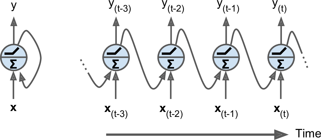
Figure 4-1. A recurrent neuron (left), unrolled through time (right)

You can easily create a layer of recurrent neurons. At each time step t, every neuron receives both the input vector x_(t) and the output vector from the previous time step y_(t–1), as shown in Figure 4-2. Note that both the inputs and outputs are vectors now (when there was just a single neuron, the output was a scalar).

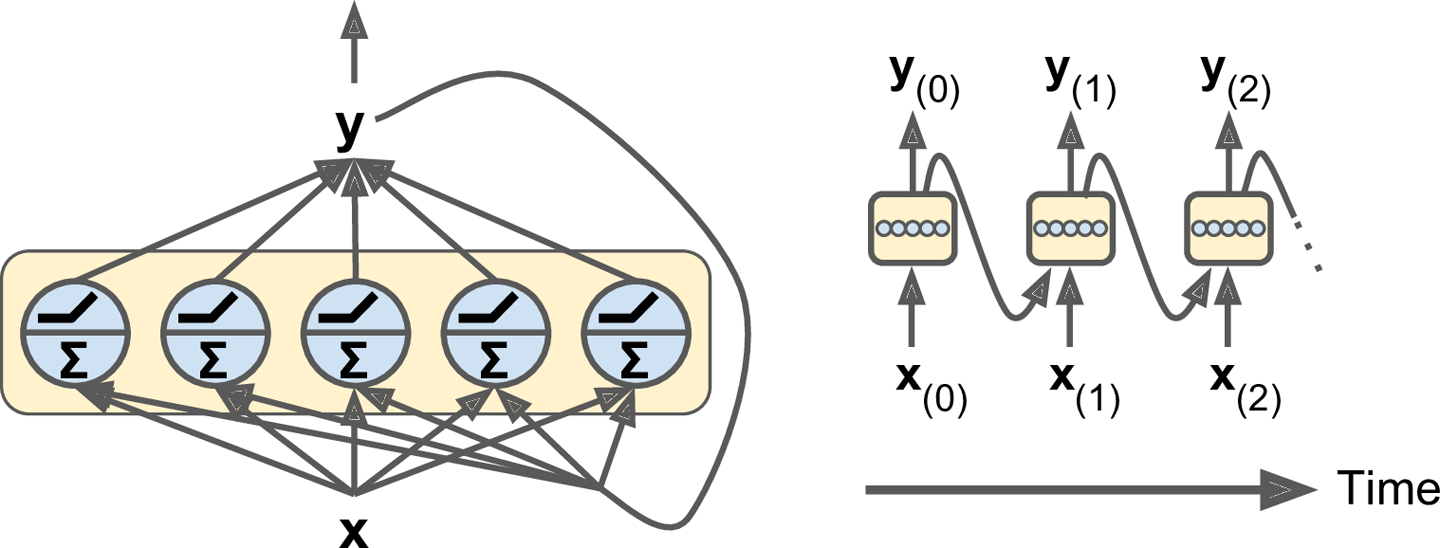
Figure 4-2. A layer of recurrent neurons (left), unrolled through time (right)

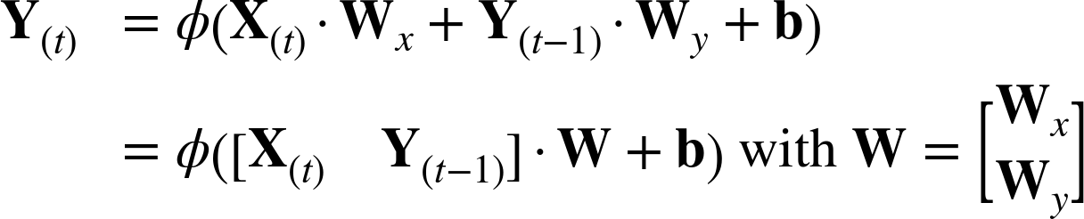
Each recurrent neuron has two sets of weights: one for the inputs x_(t) and the other for the outputs of the previous time step, y_(t–1). Let’s call these weight vectors w_x and w_y. If we consider the whole recurrent layer instead of just one recurrent neuron, we can place all the weight vectors in two weight matrices, W_x and W_y. The output vector of the whole recurrent layer can then be computed pretty much as you might expect, as shown in Equation 4-1 (b is the bias vector and ϕ(·) is the activation function, e.g., ReLU¹).

Equation 4-1. Output of a recurrent layer for a single instance

Just like for feedforward neural networks, we can compute a recurrent layer’s output in one shot for a whole mini-batch by placing all the inputs at time step t in an input matrix X_(t) (see Equation 4-2).

Equation 4-2. Outputs of a layer of recurrent neurons for all instances in a mini-batch

• Y_(t) is an m × n_neurons matrix containing the layer’s outputs at time step t for each instance in the mini-batch (m is the number of instances in the mini-batch and n_neurons is the number of neurons).

• X_(t) is an m × n_inputs matrix containing the inputs for all instances (n_inputs is the number of input features).

• W_x is an n_inputs × n_neurons matrix containing the connection weights for the inputs of the current time step.

• W_y is an n_neurons × n_neurons matrix containing the connection weights for the outputs of the previous time step.

• b is a vector of size n_neurons containing each neuron’s bias term.

• The weight matrices W_x and W_y are often concatenated vertically into a single weight matrix W of shape (n_inputs + n_neurons) × n_neurons (see the second line of Equation 4-2).

• The notation [X_(t) Y_(t–1)] represents the horizontal concatenation of the matrices X_(t) and Y_(t–1).

Notice that Y_(t) is a function of X_(t) and Y_(t–1), which is a function of X_(t–1) and Y_(t–2), which is a function of X_(t–2) and Y_(t–3), and so on. This makes Y_(t) a function of all the inputs since time t = 0 (that is, X₍₀₎, X₍₁₎, …, X_(t)). At the first time step, t = 0, there are no previous outputs, so they are typically assumed to be all zeros.

Memory Cells

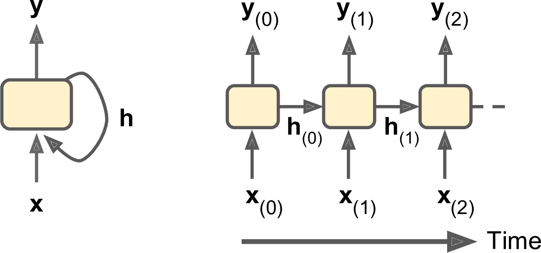
Since the output of a recurrent neuron at time step t is a function of all the inputs from previous time steps, you could say it has a form of memory. A part of a neural network that preserves some state across time steps is called a memory cell (or simply a cell). A single recurrent neuron, or a layer of recurrent neurons, is a very basic cell, but later in this chapter we will look at some more complex and powerful types of cells.

In general a cell’s state at time step t, denoted h_(t) (the “h” stands for “hidden”), is a function of some inputs at that time step and its state at the previous time step: h_(t) = f(h_(t–1), x_(t)). Its output at time step t, denoted y_(t), is also a function of the previous state and the current inputs. In the case of the basic cells we have discussed so far, the output is simply equal to the state, but in more complex cells this is not always the case, as shown in Figure 4-3.

Figure 4-3. A cell’s hidden state and its output may be different

Input and Output Sequences

An RNN can simultaneously take a sequence of inputs and produce a sequence of outputs (see Figure 4-4, top-left network). For example, this type of network is useful for predicting time series such as stock prices: you feed it the prices over the last N days, and it must output the prices shifted by one day into the future (i.e., from N – 1 days ago to tomorrow).

Alternatively, you could feed the network a sequence of inputs, and ignore all outputs except for the last one (see the top-right network). In other words, this is a sequence-to-vector network. For example, you could feed the network a sequence of words corresponding to a movie review, and the network would output a sentiment score (e.g., from –1 [hate] to +1 [love]).

Conversely, you could feed the network a single input at the first time step (and zeros for all other time steps), and let it output a sequence (see the bottom-left network). This is a vector-to-sequence network. For example, the input could be an image, and the output could be a caption for that image.

Lastly, you could have a sequence-to-vector network, called an encoder, followed by a vector-to-sequence network, called a decoder (see the bottom-right network). For example, this can be used for translating a sentence from one language to another. You would feed the network a sentence in one language, the encoder would convert this sentence into a single vector representation, and then the decoder would decode this vector into a sentence in another language. This two-step model, called an Encoder–Decoder, works much better than trying to translate on the fly with a single sequence-to-sequence RNN (like the one represented on the top left), since the last words of a sentence can affect the first words of the translation, so you need to wait until you have heard the whole sentence before translating it.

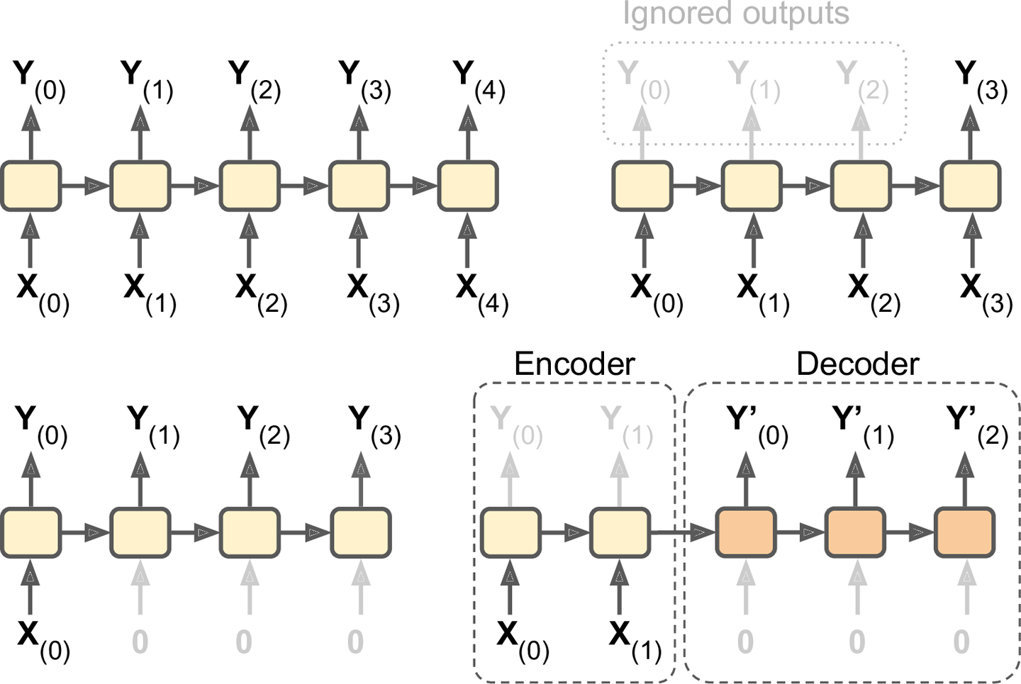
Figure 4-4. Seq to seq (top left), seq to vector (top right), vector to seq (bottom left), delayed seq to seq (bottom right)

Sounds promising, so let’s start coding!

Basic RNNs in TensorFlow

First, let’s implement a very simple RNN model, without using any of TensorFlow’s RNN operations, to better understand what goes on under the hood. We will create an RNN composed of a layer of five recurrent neurons (like the RNN represented in Figure 4-2), using the tanh activation function. We will assume that the RNN runs over only two time steps, taking input vectors of size 3 at each time step. The following code builds this RNN, unrolled through two time steps:

n_inputs = 3
n_neurons = 5

X0 = tf.placeholder(tf.float32, [None, n_inputs])
X1 = tf.placeholder(tf.float32, [None, n_inputs])

Wx = tf.Variable(tf.random_normal(shape=[n_inputs, n_neurons],dtype=tf.float32))
Wy = tf.Variable(tf.random_normal(shape=[n_neurons,n_neurons],dtype=tf.float32))
b = tf.Variable(tf.zeros([1, n_neurons], dtype=tf.float32))

Y0 = tf.tanh(tf.matmul(X0, Wx) + b)
Y1 = tf.tanh(tf.matmul(Y0, Wy) + tf.matmul(X1, Wx) + b)

init = tf.global_variables_initializer()

This network looks much like a two-layer feedforward neural network, with a few twists: first, the same weights and bias terms are shared by both layers, and second, we feed inputs at each layer, and we get outputs from each layer. To run the model, we need to feed it the inputs at both time steps, like so:

import numpy as np

# Mini-batch:        instance 0,instance 1,instance 2,instance 3
X0_batch = np.array([[0, 1, 2], [3, 4, 5], [6, 7, 8], [9, 0, 1]]) # t = 0
X1_batch = np.array([[9, 8, 7], [0, 0, 0], [6, 5, 4], [3, 2, 1]]) # t = 1

with tf.Session() as sess:
    init.run()
    Y0_val, Y1_val = sess.run([Y0, Y1], feed_dict={X0: X0_batch, X1: X1_batch})

This mini-batch contains four instances, each with an input sequence composed of exactly two inputs. At the end, Y0_val and Y1_val contain the outputs of the network at both time steps for all neurons and all instances in the mini-batch:

>>> print(Y0_val)  # output at t = 0
[[-0.0664006   0.96257669  0.68105787  0.70918542 -0.89821595]  # instance 0
 [ 0.9977755  -0.71978885 -0.99657625  0.9673925  -0.99989718]  # instance 1
 [ 0.99999774 -0.99898815 -0.99999893  0.99677622 -0.99999988]  # instance 2
 [ 1.         -1.         -1.         -0.99818915  0.99950868]] # instance 3
>>> print(Y1_val)  # output at t = 1
[[ 1.         -1.         -1.          0.40200216 -1.        ]  # instance 0
 [-0.12210433  0.62805319  0.96718419 -0.99371207 -0.25839335]  # instance 1
 [ 0.99999827 -0.9999994  -0.9999975  -0.85943311 -0.9999879 ]  # instance 2
 [ 0.99928284 -0.99999815 -0.99990582  0.98579615 -0.92205751]] # instance 3

That wasn’t too hard, but of course if you want to be able to run an RNN over 100 time steps, the graph is going to be pretty big. Now let’s look at how to create the same model using TensorFlow’s RNN operations.

Static Unrolling Through Time

The static_rnn() function creates an unrolled RNN network by chaining cells. The following code creates the exact same model as the previous one:

X0 = tf.placeholder(tf.float32, [None, n_inputs])
X1 = tf.placeholder(tf.float32, [None, n_inputs])

basic_cell = tf.contrib.rnn.BasicRNNCell(num_units=n_neurons)
output_seqs, states = tf.contrib.rnn.static_rnn(basic_cell, [X0, X1],
                                                dtype=tf.float32)
Y0, Y1 = output_seqs

First we create the input placeholders, as before. Then we create a BasicRNNCell, which you can think of as a factory that creates copies of the cell to build the unrolled RNN (one for each time step). Then we call static_rnn(), giving it the cell factory and the input tensors, and telling it the data type of the inputs (this is used to create the initial state matrix, which by default is full of zeros). The static_rnn() function calls the cell factory’s __call__() function once per input, creating two copies of the cell (each containing a layer of five recurrent neurons), with shared weights and bias terms, and it chains them just like we did earlier. The static_rnn() function returns two objects. The first is a Python list containing the output tensors for each time step. The second is a tensor containing the final states of the network. When you are using basic cells, the final state is simply equal to the last output.

If there were 50 time steps, it would not be very convenient to have to define 50 input placeholders and 50 output tensors. Moreover, at execution time you would have to feed each of the 50 placeholders and manipulate the 50 outputs. Let’s simplify this. The following code builds the same RNN again, but this time it takes a single input placeholder of shape [None, n_steps, n_inputs] where the first dimension is the mini-batch size. Then it extracts the list of input sequences for each time step. X_seqs is a Python list of n_steps tensors of shape [None, n_inputs], where once again the first dimension is the mini-batch size. To do this, we first swap the first two dimensions using the transpose() function, so that the time steps are now the first dimension. Then we extract a Python list of tensors along the first dimension (i.e., one tensor per time step) using the unstack() function. The next two lines are the same as before. Finally, we merge all the output tensors into a single tensor using the stack() function, and we swap the first two dimensions to get a final outputs tensor of shape [None, n_steps, n_neurons] (again the first dimension is the mini-batch size).

X = tf.placeholder(tf.float32, [None, n_steps, n_inputs])
X_seqs = tf.unstack(tf.transpose(X, perm=[1, 0, 2]))
basic_cell = tf.contrib.rnn.BasicRNNCell(num_units=n_neurons)
output_seqs, states = tf.contrib.rnn.static_rnn(basic_cell, X_seqs,
                                                dtype=tf.float32)
outputs = tf.transpose(tf.stack(output_seqs), perm=[1, 0, 2])

Now we can run the network by feeding it a single tensor that contains all the mini-batch sequences:

X_batch = np.array([
         # t = 0     t = 1
        [[0, 1, 2], [9, 8, 7]], # instance 0
        [[3, 4, 5], [0, 0, 0]], # instance 1
        [[6, 7, 8], [6, 5, 4]], # instance 2
        [[9, 0, 1], [3, 2, 1]], # instance 3
    ])

with tf.Session() as sess:
    init.run()
    outputs_val = outputs.eval(feed_dict={X: X_batch})

And we get a single outputs_val tensor for all instances, all time steps, and all neurons:

>>> print(outputs_val)
[[[-0.91279727  0.83698678 -0.89277941  0.80308062 -0.5283336 ]
  [-1.          1.         -0.99794829  0.99985468 -0.99273592]]

 [[-0.99994391  0.99951613 -0.9946925   0.99030769 -0.94413054]
  [ 0.48733309  0.93389565 -0.31362072  0.88573611  0.2424476 ]]

 [[-1.          0.99999875 -0.99975014  0.99956584 -0.99466234]
  [-0.99994856  0.99999434 -0.96058172  0.99784708 -0.9099462 ]]

 [[-0.95972425  0.99951482  0.96938795 -0.969908   -0.67668229]
  [-0.84596014  0.96288228  0.96856463 -0.14777924 -0.9119423 ]]]

However, this approach still builds a graph containing one cell per time step. If there were 50 time steps, the graph would look pretty ugly. It is a bit like writing a program without ever using loops (e.g., Y0=f(0, X0); Y1=f(Y0, X1); Y2=f(Y1, X2); ...; Y50=f(Y49, X50)). With such as large graph, you may even get out-of-memory (OOM) errors during backpropagation (especially with the limited memory of GPU cards), since it must store all tensor values during the forward pass so it can use them to compute gradients during the reverse pass.

Fortunately, there is a better solution: the dynamic_rnn() function.

Dynamic Unrolling Through Time

The dynamic_rnn() function uses a while_loop() operation to run over the cell the appropriate number of times, and you can set swap_memory=True if you want it to swap the GPU’s memory to the CPU’s memory during backpropagation to avoid OOM errors. Conveniently, it also accepts a single tensor for all inputs at every time step (shape [None, n_steps, n_inputs]) and it outputs a single tensor for all outputs at every time step (shape [None, n_steps, n_neurons]); there is no need to stack, unstack, or transpose. The following code creates the same RNN as earlier using the dynamic_rnn() function. It’s so much nicer!

X = tf.placeholder(tf.float32, [None, n_steps, n_inputs])

basic_cell = tf.contrib.rnn.BasicRNNCell(num_units=n_neurons)
outputs, states = tf.nn.dynamic_rnn(basic_cell, X, dtype=tf.float32)

During backpropagation, the while_loop() operation does the appropriate magic: it stores the tensor values for each iteration during the forward pass so it can use them to compute gradients during the reverse pass.

Handling Variable Length Input Sequences

So far we have used only fixed-size input sequences (all exactly two steps long). What if the input sequences have variable lengths (e.g., like sentences)? In this case you should set the sequence_length argument when calling the dynamic_rnn() (or static_rnn()) function; it must be a 1D tensor indicating the length of the input sequence for each instance. For example:

seq_length = tf.placeholder(tf.int32, [None])

[...]
outputs, states = tf.nn.dynamic_rnn(basic_cell, X, dtype=tf.float32,
                                    sequence_length=seq_length)

For example, suppose the second input sequence contains only one input instead of two. It must be padded with a zero vector in order to fit in the input tensor X (because the input tensor’s second dimension is the size of the longest sequence—i.e., 2).

X_batch = np.array([
        # step 0     step 1
        [[0, 1, 2], [9, 8, 7]], # instance 0
        [[3, 4, 5], [0, 0, 0]], # instance 1 (padded with a zero vector)
        [[6, 7, 8], [6, 5, 4]], # instance 2
        [[9, 0, 1], [3, 2, 1]], # instance 3
    ])
seq_length_batch = np.array([2, 1, 2, 2])

Of course, you now need to feed values for both placeholders X and seq_length:

with tf.Session() as sess:
    init.run()
    outputs_val, states_val = sess.run(
        [outputs, states], feed_dict={X: X_batch, seq_length: seq_length_batch})

Now the RNN outputs zero vectors for every time step past the input sequence length (look at the second instance’s output for the second time step):

>>> print(outputs_val)
[[[-0.68579948 -0.25901747 -0.80249101 -0.18141513 -0.37491536]
  [-0.99996698 -0.94501185  0.98072106 -0.9689762   0.99966913]]  # final state

 [[-0.99099374 -0.64768541 -0.67801034 -0.7415446   0.7719509 ]   # final state
  [ 0.          0.          0.          0.          0.        ]]  # zero vector

 [[-0.99978048 -0.85583007 -0.49696958 -0.93838578  0.98505187]
  [-0.99951065 -0.89148796  0.94170523 -0.38407657  0.97499216]]  # final state

 [[-0.02052618 -0.94588047  0.99935204  0.37283331  0.9998163 ]
  [-0.91052347  0.05769409  0.47446665 -0.44611037  0.89394671]]] # final state

Moreover, the states tensor contains the final state of each cell (excluding the zero vectors):

>>> print(states_val)
[[-0.99996698 -0.94501185  0.98072106 -0.9689762   0.99966913]  # t = 1
 [-0.99099374 -0.64768541 -0.67801034 -0.7415446   0.7719509 ]  # t = 0 !!!
 [-0.99951065 -0.89148796  0.94170523 -0.38407657  0.97499216]  # t = 1
 [-0.91052347  0.05769409  0.47446665 -0.44611037  0.89394671]] # t = 1

Handling Variable-Length Output Sequences

What if the output sequences have variable lengths as well? If you know in advance what length each sequence will have (for example if you know that it will be the same length as the input sequence), then you can set the sequence_length parameter as described above. Unfortunately, in general this will not be possible: for example, the length of a translated sentence is generally different from the length of the input sentence. In this case, the most common solution is to define a special output called an end-of-sequence token (EOS token). Any output past the EOS should be ignored (we will discuss this later in this chapter).

Okay, now you know how to build an RNN network (or more precisely an RNN network unrolled through time). But how do you train it?

Training RNNs

To train an RNN, the trick is to unroll it through time (like we just did) and then simply use regular backpropagation (see Figure 4-5). This strategy is called backpropagation through time (BPTT).

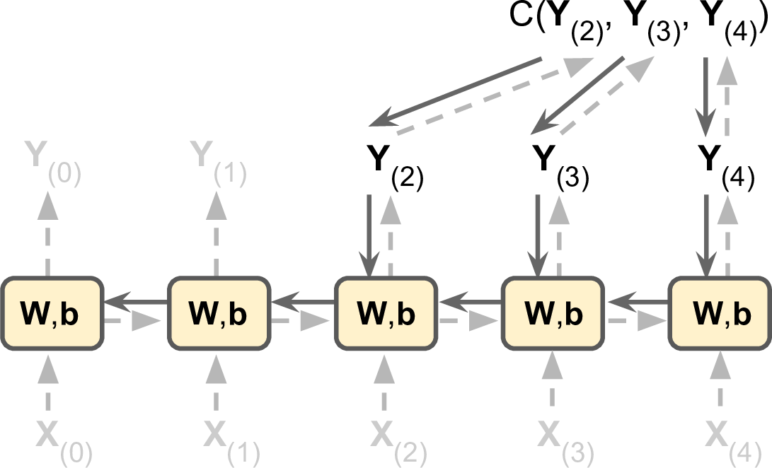
Figure 4-5. Backpropagation through time

Just like in regular backpropagation, there is a first forward pass through the unrolled network (represented by the dashed arrows); then the output sequence is evaluated using a cost function (where t_min and t_max are the first and last output time steps, not counting the ignored outputs), and the gradients of that cost function are propagated backward through the unrolled network (represented by the solid arrows); and finally the model parameters are updated using the gradients computed during BPTT. Note that the gradients flow backward through all the outputs used by the cost function, not just through the final output (for example, in Figure 4-5 the cost function is computed using the last three outputs of the network, Y₍₂₎, Y₍₃₎, and Y₍₄₎, so gradients flow through these three outputs, but not through Y₍₀₎ and Y₍₁₎). Moreover, since the same parameters W and b are used at each time step, backpropagation will do the right thing and sum over all time steps.

Training a Sequence Classifier

Let’s train an RNN to classify MNIST images. A convolutional neural network would be better suited for image classification (see Chapter 3), but this makes for a simple example that you are already familiar with. We will treat each image as a sequence of 28 rows of 28 pixels each (since each MNIST image is 28 × 28 pixels). We will use cells of 150 recurrent neurons, plus a fully connected layer containing 10 neurons (one per class) connected to the output of the last time step, followed by a softmax layer (see Figure 4-6).

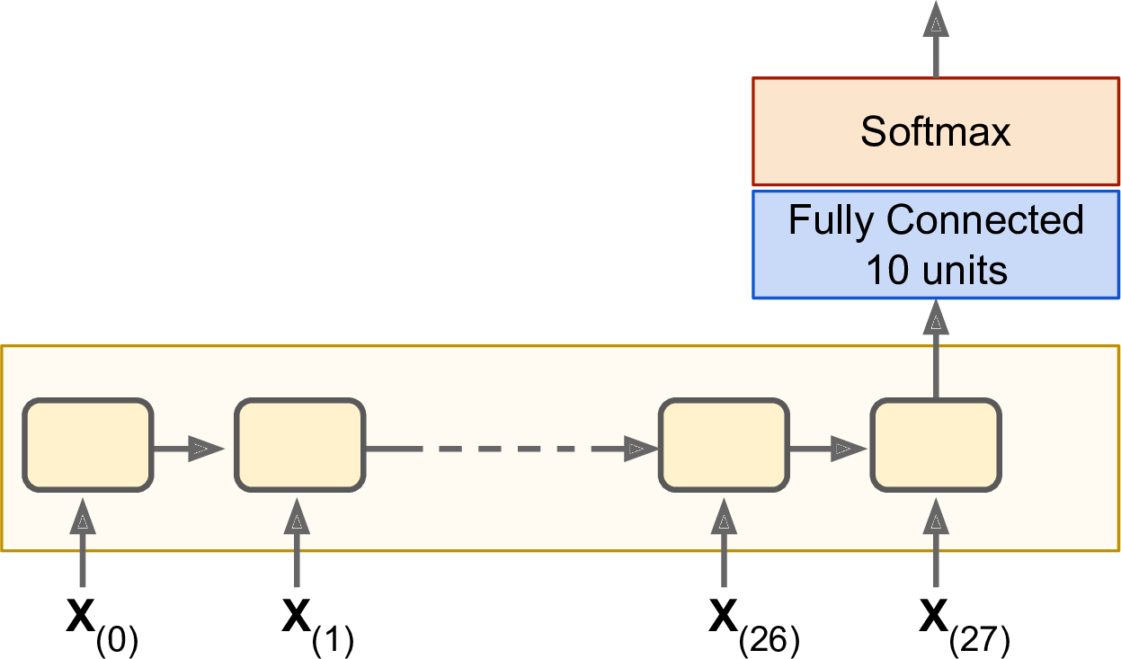
Figure 4-6. Sequence classifier

The construction phase is quite straightforward; it’s pretty much the same as the MNIST classifier we built in Chapter 1 except that an unrolled RNN replaces the hidden layers. Note that the fully connected layer is connected to the states tensor, which contains only the final state of the RNN (i.e., the 28^th output). Also note that y is a placeholder for the target classes.

n_steps = 28
n_inputs = 28
n_neurons = 150
n_outputs = 10

learning_rate = 0.001

X = tf.placeholder(tf.float32, [None, n_steps, n_inputs])
y = tf.placeholder(tf.int32, [None])

basic_cell = tf.contrib.rnn.BasicRNNCell(num_units=n_neurons)
outputs, states = tf.nn.dynamic_rnn(basic_cell, X, dtype=tf.float32)

logits = tf.layers.dense(states, n_outputs)
xentropy = tf.nn.sparse_softmax_cross_entropy_with_logits(labels=y,
                                                          logits=logits)
loss = tf.reduce_mean(xentropy)
optimizer = tf.train.AdamOptimizer(learning_rate=learning_rate)
training_op = optimizer.minimize(loss)
correct = tf.nn.in_top_k(logits, y, 1)
accuracy = tf.reduce_mean(tf.cast(correct, tf.float32))

init = tf.global_variables_initializer()

Now let’s load the MNIST data and reshape the test data to [batch_size, n_steps, n_inputs] as is expected by the network. We will take care of reshaping the training data in a moment.

from tensorflow.examples.tutorials.mnist import input_data

mnist = input_data.read_data_sets("/tmp/data/")
X_test = mnist.test.images.reshape((-1, n_steps, n_inputs))
y_test = mnist.test.labels

Now we are ready to train the RNN. The execution phase is exactly the same as for the MNIST classifier in Chapter 1, except that we reshape each training batch before feeding it to the network.

n_epochs = 100
batch_size = 150

with tf.Session() as sess:
    init.run()
    for epoch in range(n_epochs):
        for iteration in range(mnist.train.num_examples // batch_size):
            X_batch, y_batch = mnist.train.next_batch(batch_size)
            X_batch = X_batch.reshape((-1, n_steps, n_inputs))
            sess.run(training_op, feed_dict={X: X_batch, y: y_batch})
        acc_train = accuracy.eval(feed_dict={X: X_batch, y: y_batch})
        acc_test = accuracy.eval(feed_dict={X: X_test, y: y_test})
        print(epoch, "Train accuracy:", acc_train, "Test accuracy:", acc_test)

The output should look like this:

0 Train accuracy: 0.94 Test accuracy: 0.9308
1 Train accuracy: 0.933333 Test accuracy: 0.9431
[...]
98 Train accuracy: 0.98 Test accuracy: 0.9794
99 Train accuracy: 1.0 Test accuracy: 0.9804

We get over 98% accuracy—not bad! Plus you would certainly get a better result by tuning the hyperparameters, initializing the RNN weights using He initialization, training longer, or adding a bit of regularization (e.g., dropout).

You can specify an initializer for the RNN by wrapping its construction code in a variable scope (e.g., use variable_scope("rnn", initializer=variance_scaling_initializer()) to use He initialization).

Training to Predict Time Series

Now let’s take a look at how to handle time series, such as stock prices, air temperature, brain wave patterns, and so on. In this section we will train an RNN to predict the next value in a generated time series. Each training instance is a randomly selected sequence of 20 consecutive values from the time series, and the target sequence is the same as the input sequence, except it is shifted by one time step into the future (see Figure 4-7).

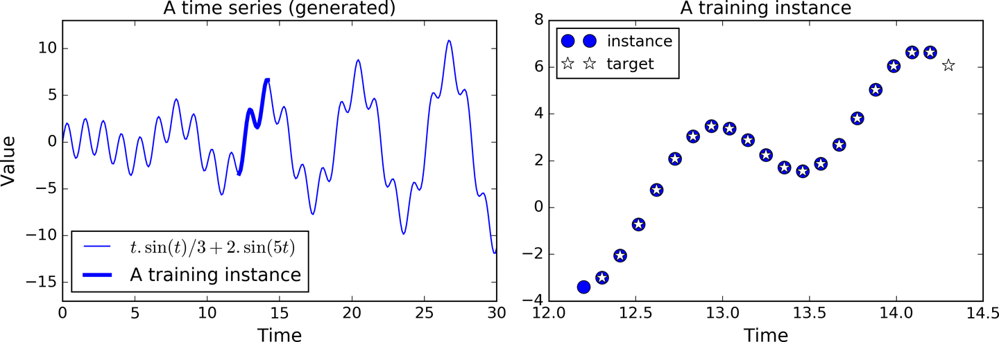
Figure 4-7. Time series (left), and a training instance from that series (right)

First, let’s create the RNN. It will contain 100 recurrent neurons and we will unroll it over 20 time steps since each training instance will be 20 inputs long. Each input will contain only one feature (the value at that time). The targets are also sequences of 20 inputs, each containing a single value. The code is almost the same as earlier:

n_steps = 20
n_inputs = 1
n_neurons = 100
n_outputs = 1

X = tf.placeholder(tf.float32, [None, n_steps, n_inputs])
y = tf.placeholder(tf.float32, [None, n_steps, n_outputs])
cell = tf.contrib.rnn.BasicRNNCell(num_units=n_neurons, activation=tf.nn.relu)
outputs, states = tf.nn.dynamic_rnn(cell, X, dtype=tf.float32)

In general you would have more than just one input feature. For example, if you were trying to predict stock prices, you would likely have many other input features at each time step, such as prices of competing stocks, ratings from analysts, or any other feature that might help the system make its predictions.

At each time step we now have an output vector of size 100. But what we actually want is a single output value at each time step. The simplest solution is to wrap the cell in an OutputProjectionWrapper. A cell wrapper acts like a normal cell, proxying every method call to an underlying cell, but it also adds some functionality. The OutputProjectionWrapper adds a fully connected layer of linear neurons (i.e., without any activation function) on top of each output (but it does not affect the cell state). All these fully connected layers share the same (trainable) weights and bias terms. The resulting RNN is represented in Figure 4-8.

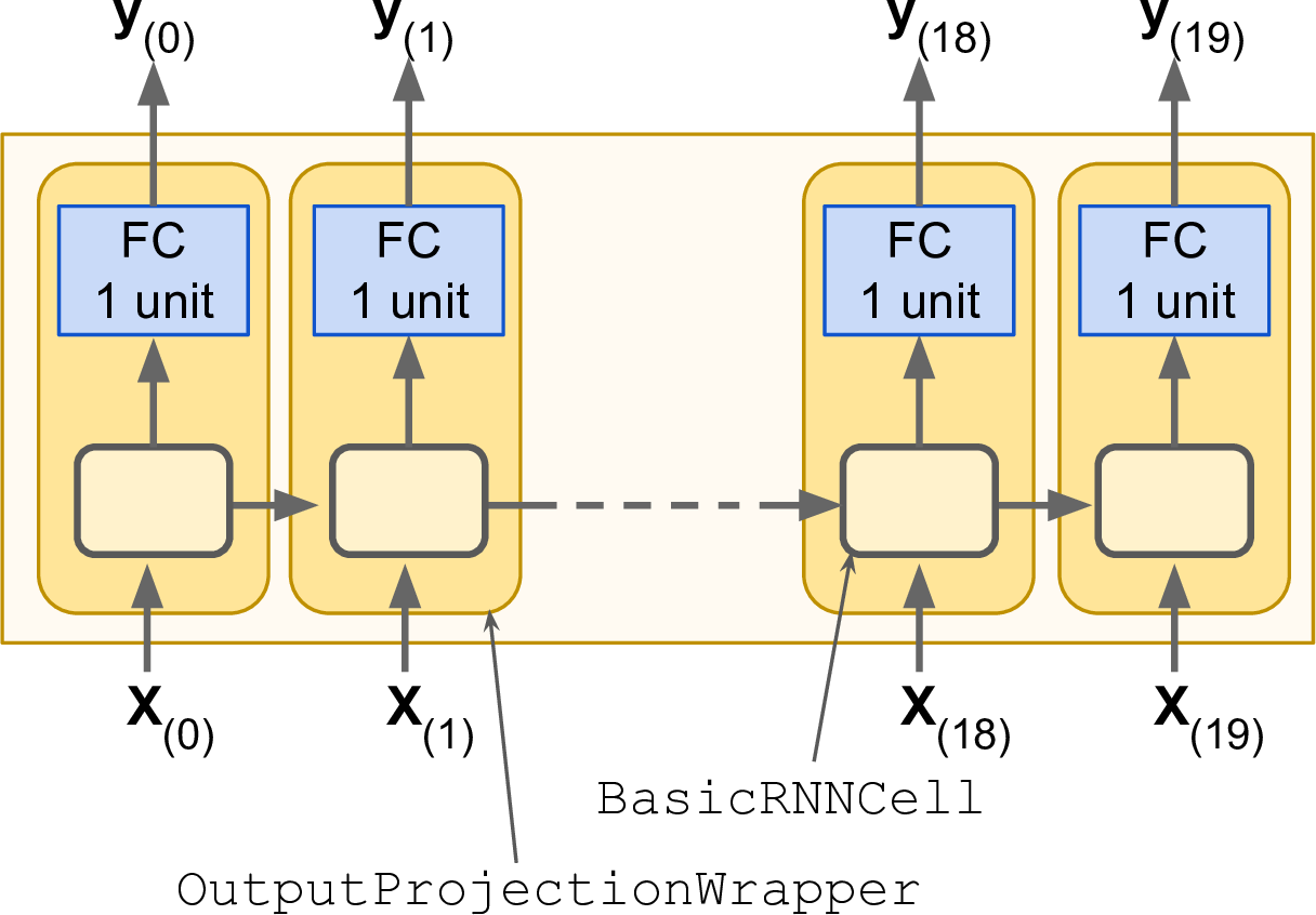
Figure 4-8. RNN cells using output projections

Wrapping a cell is quite easy. Let’s tweak the preceding code by wrapping the BasicRNNCell into an OutputProjectionWrapper:

cell = tf.contrib.rnn.OutputProjectionWrapper(
    tf.contrib.rnn.BasicRNNCell(num_units=n_neurons, activation=tf.nn.relu),
    output_size=n_outputs)

So far, so good. Now we need to define the cost function. We will use the Mean Squared Error (MSE), as we did in previous regression tasks. Next we will create an Adam optimizer, the training op, and the variable initialization op, as usual:

learning_rate = 0.001

loss = tf.reduce_mean(tf.square(outputs - y))
optimizer = tf.train.AdamOptimizer(learning_rate=learning_rate)
training_op = optimizer.minimize(loss)

init = tf.global_variables_initializer()

Now on to the execution phase:

n_iterations = 1500
batch_size = 50

with tf.Session() as sess:
    init.run()
    for iteration in range(n_iterations):
        X_batch, y_batch = [...]  # fetch the next training batch
        sess.run(training_op, feed_dict={X: X_batch, y: y_batch})
        if iteration % 100 == 0:
            mse = loss.eval(feed_dict={X: X_batch, y: y_batch})
            print(iteration, "\tMSE:", mse)

The program’s output should look like this:

0       MSE: 13.6543
100     MSE: 0.538476
200     MSE: 0.168532
300     MSE: 0.0879579
400     MSE: 0.0633425
[...]

Once the model is trained, you can make predictions:

X_new = [...]  # New sequences
y_pred = sess.run(outputs, feed_dict={X: X_new})

Figure 4-9 shows the predicted sequence for the instance we looked at earlier (in Figure 4-7), after just 1,000 training iterations.

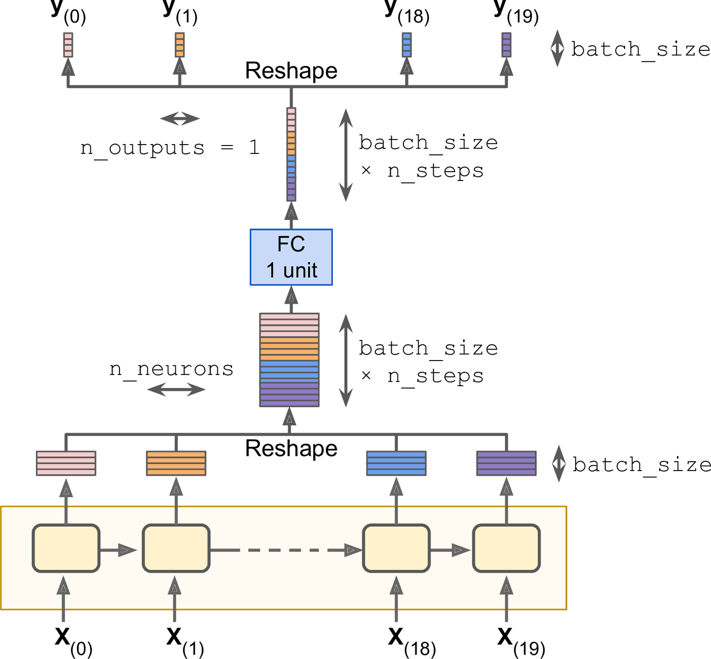
Although using an OutputProjectionWrapper is the simplest solution to reduce the dimensionality of the RNN’s output sequences down to just one value per time step (per instance), it is not the most efficient. There is a trickier but more efficient solution: you can reshape the RNN outputs from [batch_size, n_steps, n_neurons] to [batch_size * n_steps, n_neurons], then apply a single fully connected layer with the appropriate output size (in our case just 1), which will result in an output tensor of shape [batch_size * n_steps, n_outputs], and then reshape this tensor to [batch_size, n_steps, n_outputs]. These operations are represented in Figure 4-10.

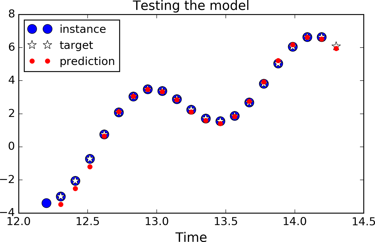
Figure 4-9. Time series prediction

Figure 4-10. Stack all the outputs, apply the projection, then unstack the result

To implement this solution, we first revert to a basic cell, without the OutputProjectionWrapper:

cell = tf.contrib.rnn.BasicRNNCell(num_units=n_neurons, activation=tf.nn.relu)
rnn_outputs, states = tf.nn.dynamic_rnn(cell, X, dtype=tf.float32)

Then we stack all the outputs using the reshape() operation, apply the fully connected linear layer (without using any activation function; this is just a projection), and finally unstack all the outputs, again using reshape():

stacked_rnn_outputs = tf.reshape(rnn_outputs, [-1, n_neurons])
stacked_outputs = tf.layers.dense(stacked_rnn_outputs, n_outputs)
outputs = tf.reshape(stacked_outputs, [-1, n_steps, n_outputs])

The rest of the code is the same as earlier. This can provide a significant speed boost since there is just one fully connected layer instead of one per time step.

Creative RNN

Now that we have a model that can predict the future, we can use it to generate some creative sequences, as explained at the beginning of the chapter. All we need is to provide it a seed sequence containing n_steps values (e.g., full of zeros), use the model to predict the next value, append this predicted value to the sequence, feed the last n_steps values to the model to predict the next value, and so on. This process generates a new sequence that has some resemblance to the original time series (see Figure 4-11).

sequence = [0.] * n_steps
for iteration in range(300):
    X_batch = np.array(sequence[-n_steps:]).reshape(1, n_steps, 1)
    y_pred = sess.run(outputs, feed_dict={X: X_batch})
    sequence.append(y_pred[0, -1, 0])

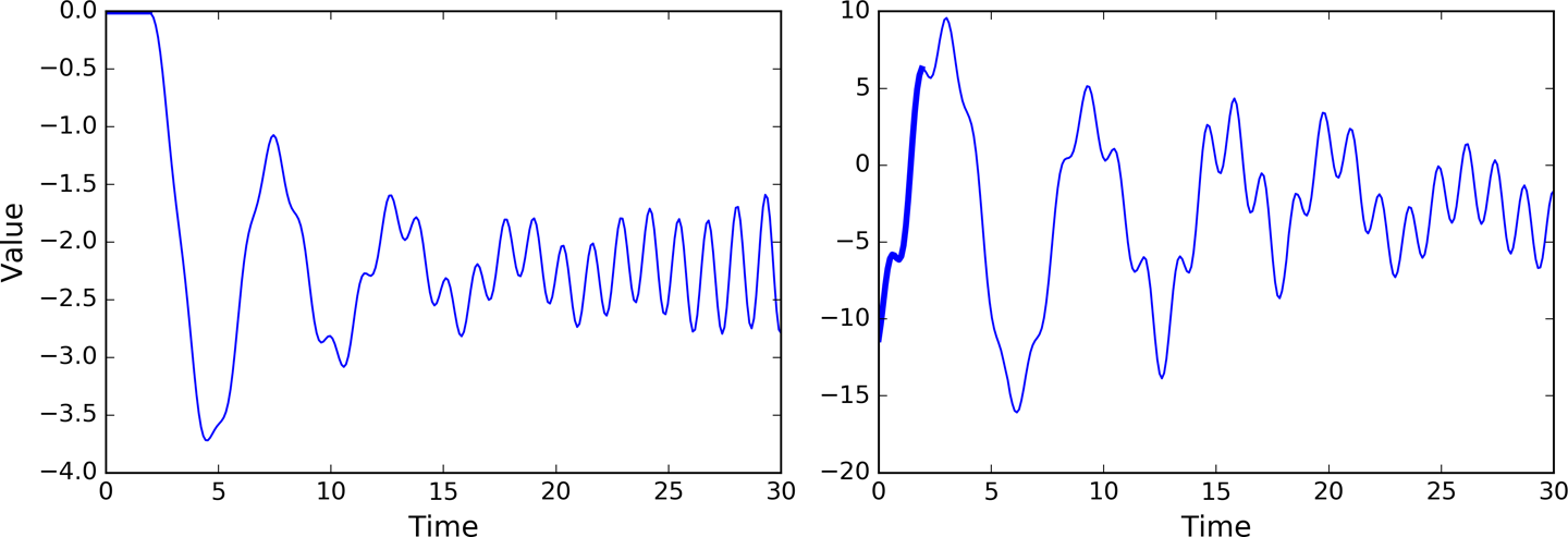
Figure 4-11. Creative sequences, seeded with zeros (left) or with an instance (right)

Now you can try to feed all your John Lennon albums to an RNN and see if it can generate the next “Imagine.” However, you will probably need a much more powerful RNN, with more neurons, and also much deeper. Let’s look at deep RNNs now.

Deep RNNs

It is quite common to stack multiple layers of cells, as shown in Figure 4-12. This gives you a deep RNN.

To implement a deep RNN in TensorFlow, you can create several cells and stack them into a MultiRNNCell. In the following code we stack three identical cells (but you could very well use various kinds of cells with a different number of neurons):

n_neurons = 100
n_layers = 3

layers = [tf.contrib.rnn.BasicRNNCell(num_units=n_neurons,
                                      activation=tf.nn.relu)
          for layer in range(n_layers)]
multi_layer_cell = tf.contrib.rnn.MultiRNNCell(layers)
outputs, states = tf.nn.dynamic_rnn(multi_layer_cell, X, dtype=tf.float32)

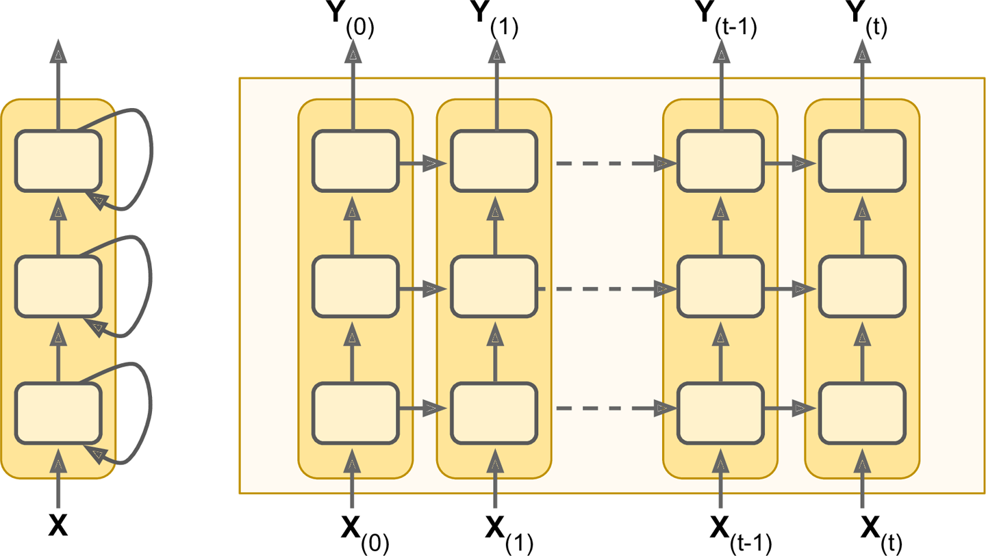
Figure 4-12. Deep RNN (left), unrolled through time (right)

That’s all there is to it! The states variable is a tuple containing one tensor per layer, each representing the final state of that layer’s cell (with shape [batch_size, n_neurons]). If you set state_is_tuple=False when creating the MultiRNNCell, then states becomes a single tensor containing the states from every layer, concatenated along the column axis (i.e., its shape is [batch_size, n_layers * n_neurons]). Note that before TensorFlow 0.11.0, this behavior was the default.

Distributing a Deep RNN Across Multiple GPUs

We can efficiently distribute deep RNNs across multiple GPUs by pinning each layer to a different GPU. However, if you try to create each cell in a different device() block, it will not work:

with tf.device("/gpu:0"):  # BAD! This is ignored.
    layer1 = tf.contrib.rnn.BasicRNNCell(num_units=n_neurons)

with tf.device("/gpu:1"):  # BAD! Ignored again.
    layer2 = tf.contrib.rnn.BasicRNNCell(num_units=n_neurons)

This fails because a BasicRNNCell is a cell factory, not a cell per se (as mentioned earlier); no cells get created when you create the factory, and thus no variables do either. The device block is simply ignored. The cells actually get created later. When you call dynamic_rnn(), it calls the MultiRNNCell, which calls each individual BasicRNNCell, which create the actual cells (including their variables). Unfortunately, none of these classes provide any way to control the devices on which the variables get created. If you try to put the dynamic_rnn() call within a device block, the whole RNN gets pinned to a single device. So are you stuck? Fortunately not! The trick is to create your own cell wrapper (or use the tf.contrib.rnn.DeviceWrapper class, which was added in TensorFlow 1.1):

import tensorflow as tf

class DeviceCellWrapper(tf.contrib.rnn.RNNCell):
  def __init__(self, device, cell):
    self._cell = cell
    self._device = device

  @property
  def state_size(self):
    return self._cell.state_size

  @property
  def output_size(self):
    return self._cell.output_size

  def __call__(self, inputs, state, scope=None):
    with tf.device(self._device):
        return self._cell(inputs, state, scope)

This wrapper simply proxies every method call to another cell, except it wraps the __call__() function within a device block.² Now you can distribute each layer on a different GPU:

devices = ["/gpu:0", "/gpu:1", "/gpu:2"]
cells = [DeviceCellWrapper(dev,tf.contrib.rnn.BasicRNNCell(num_units=n_neurons))
         for dev in devices]
multi_layer_cell = tf.contrib.rnn.MultiRNNCell(cells)
outputs, states = tf.nn.dynamic_rnn(multi_layer_cell, X, dtype=tf.float32)

Do not set state_is_tuple=False, or the MultiRNNCell will concatenate all the cell states into a single tensor, on a single GPU.

Applying Dropout

If you build a very deep RNN, it may end up overfitting the training set. To prevent that, a common technique is to apply dropout (introduced in Chapter 2). You can simply add a dropout layer before or after the RNN as usual, but if you also want to apply dropout between the RNN layers, you need to use a DropoutWrapper. The following code applies dropout to the inputs of each layer in the RNN:

keep_prob = tf.placeholder_with_default(1.0, shape=())

cells = [tf.contrib.rnn.BasicRNNCell(num_units=n_neurons)
         for layer in range(n_layers)]
cells_drop = [tf.contrib.rnn.DropoutWrapper(cell, input_keep_prob=keep_prob)
              for cell in cells]
multi_layer_cell = tf.contrib.rnn.MultiRNNCell(cells_drop)
rnn_outputs, states = tf.nn.dynamic_rnn(multi_layer_cell, X, dtype=tf.float32)
# The rest of the construction phase is just like earlier.

During training, you can feed any value you want to the keep_prob placeholder (typically, 0.5):

n_iterations = 1500
batch_size = 50
train_keep_prob = 0.5

with tf.Session() as sess:
    init.run()
    for iteration in range(n_iterations):
        X_batch, y_batch = next_batch(batch_size, n_steps)
        _, mse = sess.run([training_op, loss],
                          feed_dict={X: X_batch, y: y_batch,
                                     keep_prob: train_keep_prob})
    saver.save(sess, "./my_dropout_time_series_model")

During testing, you should let keep_prob default to 1.0, effectively turning dropout off (remember that it should only be active during training):

with tf.Session() as sess:
    saver.restore(sess, "./my_dropout_time_series_model")

    X_new = [...] # some test data
    y_pred = sess.run(outputs, feed_dict={X: X_new})

Note that it is also possible to apply dropout to the outputs by setting output_keep_prob, and since TensorFlow 1.1, it is also possible to apply dropout to the cell’s state using state_keep_prob.

With that you should be able to train all sorts of RNNs! Unfortunately, if you want to train an RNN on long sequences, things will get a bit harder. Let’s see why and what you can do about it.

The Difficulty of Training over Many Time Steps

To train an RNN on long sequences, you will need to run it over many time steps, making the unrolled RNN a very deep network. Just like any deep neural network it may suffer from the vanishing/exploding gradients problem (discussed in Chapter 2) and take forever to train. Many of the tricks we discussed to alleviate this problem can be used for deep unrolled RNNs as well: good parameter initialization, nonsaturating activation functions (e.g., ReLU), Batch Normalization, Gradient Clipping, and faster optimizers. However, if the RNN needs to handle even moderately long sequences (e.g., 100 inputs), then training will still be very slow.

The simplest and most common solution to this problem is to unroll the RNN only over a limited number of time steps during training. This is called truncated backpropagation through time. In TensorFlow you can implement it simply by truncating the input sequences. For example, in the time series prediction problem, you would simply reduce n_steps during training. The problem, of course, is that the model will not be able to learn long-term patterns. One workaround could be to make sure that these shortened sequences contain both old and recent data, so that the model can learn to use both (e.g., the sequence could contain monthly data for the last five months, then weekly data for the last five weeks, then daily data over the last five days). But this workaround has its limits: what if fine-grained data from last year is actually useful? What if there was a brief but significant event that absolutely must be taken into account, even years later (e.g., the result of an election)?

Besides the long training time, a second problem faced by long-running RNNs is the fact that the memory of the first inputs gradually fades away. Indeed, due to the transformations that the data goes through when traversing an RNN, some information is lost after each time step. After a while, the RNN’s state contains virtually no trace of the first inputs. This can be a showstopper. For example, say you want to perform sentiment analysis on a long review that starts with the four words “I loved this movie,” but the rest of the review lists the many things that could have made the movie even better. If the RNN gradually forgets the first four words, it will completely misinterpret the review. To solve this problem, various types of cells with long-term memory have been introduced. They have proved so successful that the basic cells are not much used anymore. Let’s first look at the most popular of these long memory cells: the LSTM cell.

LSTM Cell

The Long Short-Term Memory (LSTM) cell was proposed in 1997³ by Sepp Hochreiter and Jürgen Schmidhuber, and it was gradually improved over the years by several researchers, such as Alex Graves, Haşim Sak,⁴ Wojciech Zaremba,⁵ and many more. If you consider the LSTM cell as a black box, it can be used very much like a basic cell, except it will perform much better; training will converge faster and it will detect long-term dependencies in the data. In TensorFlow, you can simply use a BasicLSTMCell instead of a BasicRNNCell:

lstm_cell = tf.contrib.rnn.BasicLSTMCell(num_units=n_neurons)

LSTM cells manage two state vectors, and for performance reasons they are kept separate by default. You can change this default behavior by setting state_is_tuple=False when creating the BasicLSTMCell.

So how does an LSTM cell work? The architecture of a basic LSTM cell is shown in Figure 4-13.

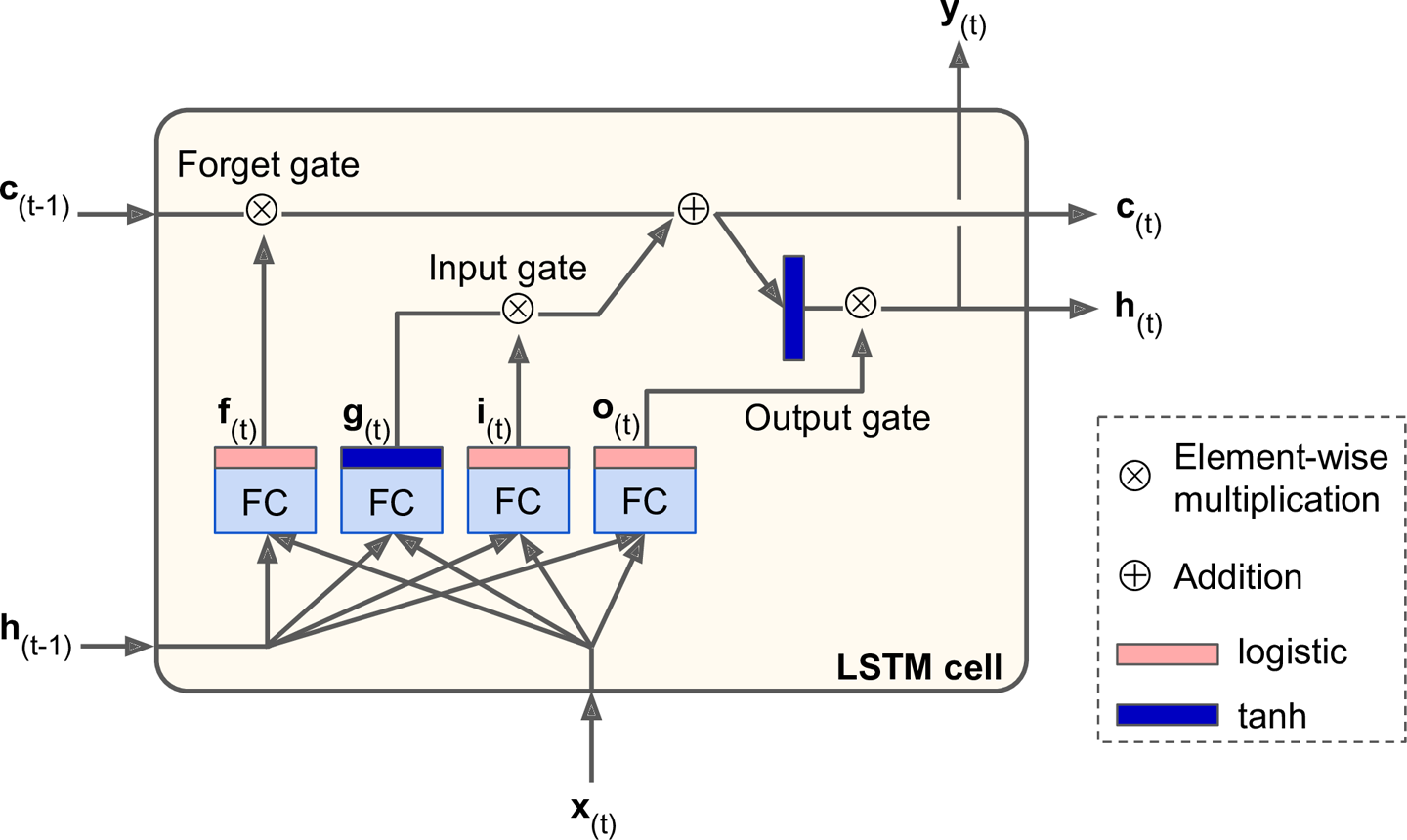
Figure 4-13. LSTM cell

If you don’t look at what’s inside the box, the LSTM cell looks exactly like a regular cell, except that its state is split in two vectors: h_(t) and c_(t) (“c” stands for “cell”). You can think of h_(t) as the short-term state and c_(t) as the long-term state.

Now let’s open the box! The key idea is that the network can learn what to store in the long-term state, what to throw away, and what to read from it. As the long-term state c_(t–1) traverses the network from left to right, you can see that it first goes through a forget gate, dropping some memories, and then it adds some new memories via the addition operation (which adds the memories that were selected by an input gate). The result c_(t) is sent straight out, without any further transformation. So, at each time step, some memories are dropped and some memories are added. Moreover, after the addition operation, the long-term state is copied and passed through the tanh function, and then the result is filtered by the output gate. This produces the short-term state h_(t) (which is equal to the cell’s output for this time step y_(t)). Now let’s look at where new memories come from and how the gates work.

First, the current input vector x_(t) and the previous short-term state h_(t–1) are fed to four different fully connected layers. They all serve a different purpose:

• The main layer is the one that outputs g_(t). It has the usual role of analyzing the current inputs x_(t) and the previous (short-term) state h_(t–1). In a basic cell, there is nothing else than this layer, and its output goes straight out to y_(t) and h_(t). In contrast, in an LSTM cell this layer’s output does not go straight out, but instead it is partially stored in the long-term state.

• The three other layers are gate controllers. Since they use the logistic activation function, their outputs range from 0 to 1. As you can see, their outputs are fed to element-wise multiplication operations, so if they output 0s, they close the gate, and if they output 1s, they open it. Specifically:

  • The forget gate (controlled by f_(t)) controls which parts of the long-term state should be erased.

  • The input gate (controlled by i_(t)) controls which parts of g_(t) should be added to the long-term state (this is why we said it was only “partially stored”).

  • Finally, the output gate (controlled by o_(t)) controls which parts of the long-term state should be read and output at this time step (both to h_(t)) and y_(t).

In short, an LSTM cell can learn to recognize an important input (that’s the role of the input gate), store it in the long-term state, learn to preserve it for as long as it is needed (that’s the role of the forget gate), and learn to extract it whenever it is needed. This explains why they have been amazingly successful at capturing long-term patterns in time series, long texts, audio recordings, and more.

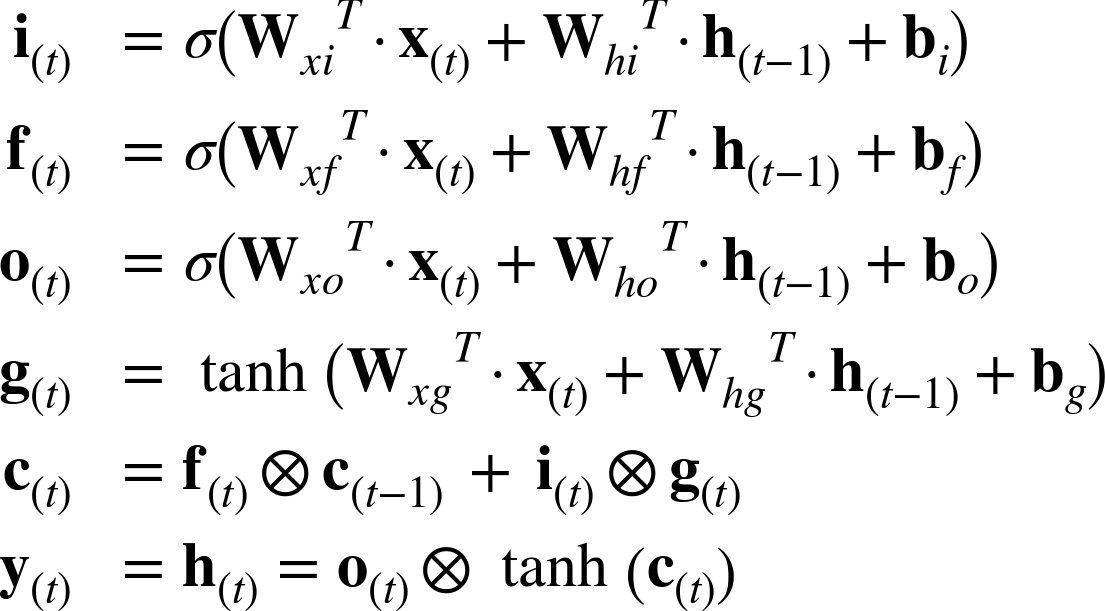
Equation 4-3 summarizes how to compute the cell’s long-term state, its short-term state, and its output at each time step for a single instance (the equations for a whole mini-batch are very similar).

Equation 4-3. LSTM computations

• W_xi, W_xf, W_xo, W_xg are the weight matrices of each of the four layers for their connection to the input vector x_(t).

• W_hi, W_hf, W_ho, and W_hg are the weight matrices of each of the four layers for their connection to the previous short-term state h_(t–1).

• b_i, b_f, b_o, and b_g are the bias terms for each of the four layers. Note that TensorFlow initializes b_f to a vector full of 1s instead of 0s. This prevents forgetting everything at the beginning of training.

Peephole Connections

In a basic LSTM cell, the gate controllers can look only at the input x_(t) and the previous short-term state h_(t–1). It may be a good idea to give them a bit more context by letting them peek at the long-term state as well. This idea was proposed by Felix Gers and Jürgen Schmidhuber in 2000.⁶ They proposed an LSTM variant with extra connections called peephole connections: the previous long-term state c_(t–1) is added as an input to the controllers of the forget gate and the input gate, and the current long-term state c_(t) is added as input to the controller of the output gate.

To implement peephole connections in TensorFlow, you must use the LSTMCell instead of the BasicLSTMCell and set use_peepholes=True:

lstm_cell = tf.contrib.rnn.LSTMCell(num_units=n_neurons, use_peepholes=True)

There are many other variants of the LSTM cell. One particularly popular variant is the GRU cell, which we will look at now.

GRU Cell

The Gated Recurrent Unit (GRU) cell (see Figure 4-14) was proposed by Kyunghyun Cho et al. in a 2014 paper⁷ that also introduced the Encoder–Decoder network we mentioned earlier.

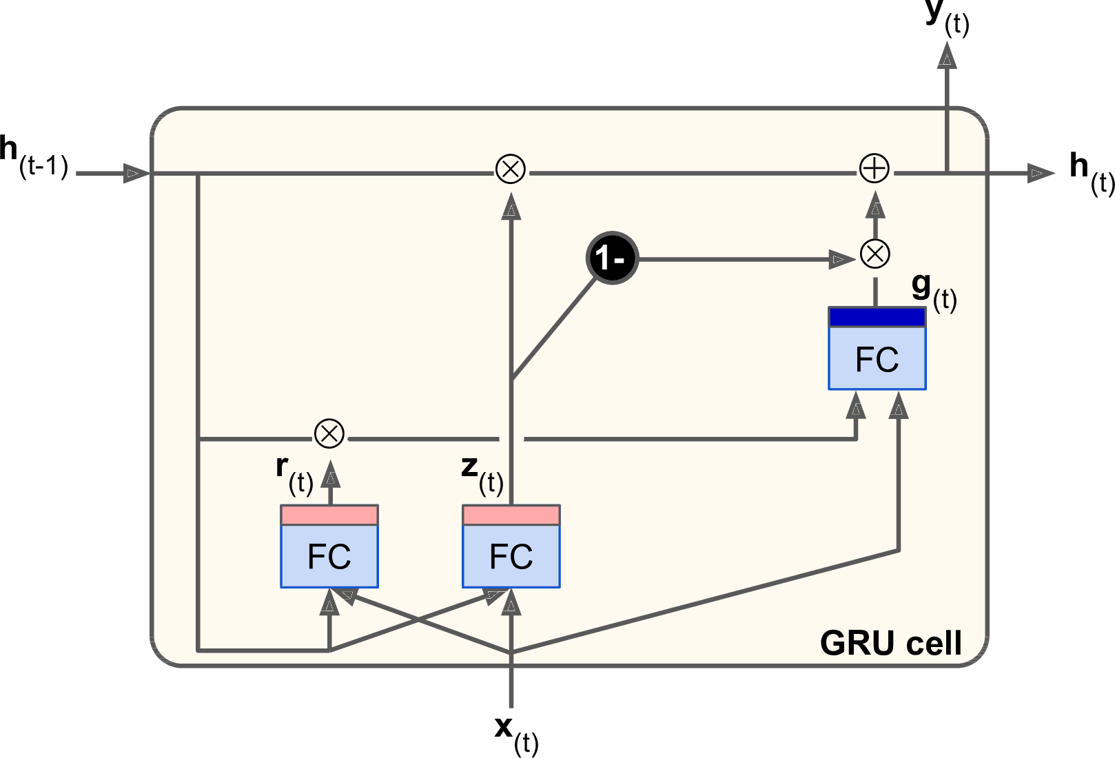
Figure 4-14. GRU cell

The GRU cell is a simplified version of the LSTM cell, and it seems to perform just as well⁸ (which explains its growing popularity). The main simplifications are:

• Both state vectors are merged into a single vector h_(t).

• A single gate controller controls both the forget gate and the input gate. If the gate controller outputs a 1, the forget gate is open and the input gate is closed. If it outputs a 0, the opposite happens. In other words, whenever a memory must be stored, the location where it will be stored is erased first. This is actually a frequent variant to the LSTM cell in and of itself.

• There is no output gate; the full state vector is output at every time step. However, there is a new gate controller that controls which part of the previous state will be shown to the main layer.

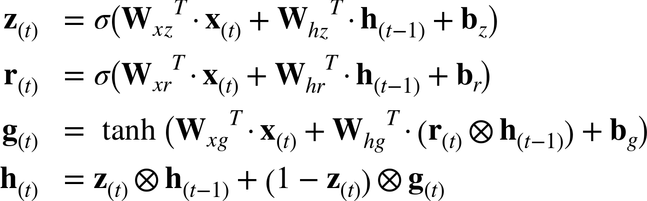
Equation 4-4 summarizes how to compute the cell’s state at each time step for a single instance.

Equation 4-4. GRU computations

Creating a GRU cell in TensorFlow is trivial:

gru_cell = tf.contrib.rnn.GRUCell(num_units=n_neurons)

LSTM or GRU cells are one of the main reasons behind the success of RNNs in recent years, in particular for applications in natural language processing (NLP).

Natural Language Processing

Most of the state-of-the-art NLP applications, such as machine translation, automatic summarization, parsing, sentiment analysis, and more, are now based (at least in part) on RNNs. In this last section, we will take a quick look at what a machine translation model looks like. This topic is very well covered by TensorFlow’s awesome Word2Vec and Seq2Seq tutorials, so you should definitely check them out.

Word Embeddings

Before we start, we need to choose a word representation. One option could be to represent each word using a one-hot vector. Suppose your vocabulary contains 50,000 words, then the n^th word would be represented as a 50,000-dimensional vector, full of 0s except for a 1 at the n^th position. However, with such a large vocabulary, this sparse representation would not be efficient at all. Ideally, you want similar words to have similar representations, making it easy for the model to generalize what it learns about a word to all similar words. For example, if the model is told that “I drink milk” is a valid sentence, and if it knows that “milk” is close to “water” but far from “shoes,” then it will know that “I drink water” is probably a valid sentence as well, while “I drink shoes” is probably not. But how can you come up with such a meaningful representation?

The most common solution is to represent each word in the vocabulary using a fairly small and dense vector (e.g., 150 dimensions), called an embedding, and just let the neural network learn a good embedding for each word during training. At the beginning of training, embeddings are simply chosen randomly, but during training, backpropagation automatically moves the embeddings around in a way that helps the neural network perform its task. Typically this means that similar words will gradually cluster close to one another, and even end up organized in a rather meaningful way. For example, embeddings may end up placed along various axes that represent gender, singular/plural, adjective/noun, and so on. The result can be truly amazing.⁹

In TensorFlow, you first need to create the variable representing the embeddings for every word in your vocabulary (initialized randomly):

vocabulary_size = 50000
embedding_size = 150

init_embeds = tf.random_uniform([vocabulary_size, embedding_size], -1.0, 1.0)
embeddings = tf.Variable(init_embeds)

Now suppose you want to feed the sentence “I drink milk” to your neural network. You should first preprocess the sentence and break it into a list of known words. For example you may remove unnecessary characters, replace unknown words by a predefined token word such as “[UNK]”, replace numerical values by “[NUM]”, replace URLs by “[URL]”, and so on. Once you have a list of known words, you can look up each word’s integer identifier (from 0 to 49999) in a dictionary, for example [72, 3335, 288]. At that point, you are ready to feed these word identifiers to TensorFlow using a placeholder, and apply the embedding_lookup() function to get the corresponding embeddings:

train_inputs = tf.placeholder(tf.int32, shape=[None])  # from ids...
embed = tf.nn.embedding_lookup(embeddings, train_inputs)  # ...to embeddings

Once your model has learned good word embeddings, they can actually be reused fairly efficiently in any NLP application: after all, “milk” is still close to “water” and far from “shoes” no matter what your application is. In fact, instead of training your own word embeddings, you may want to download pretrained word embeddings. Just like when reusing pretrained layers (see Chapter 2), you can choose to freeze the pretrained embeddings (e.g., creating the embeddings variable using trainable=False) or let backpropagation tweak them for your application. The first option will speed up training, but the second may lead to slightly higher performance.

Embeddings are also useful for representing categorical attributes that can take on a large number of different values, especially when there are complex similarities between values. For example, consider professions, hobbies, dishes, species, brands, and so on.

You now have almost all the tools you need to implement a machine translation system. Let’s look at this now.

An Encoder–Decoder Network for Machine Translation

Let’s take a look at a simple machine translation model¹⁰ that will translate English sentences to French (see Figure 4-15).

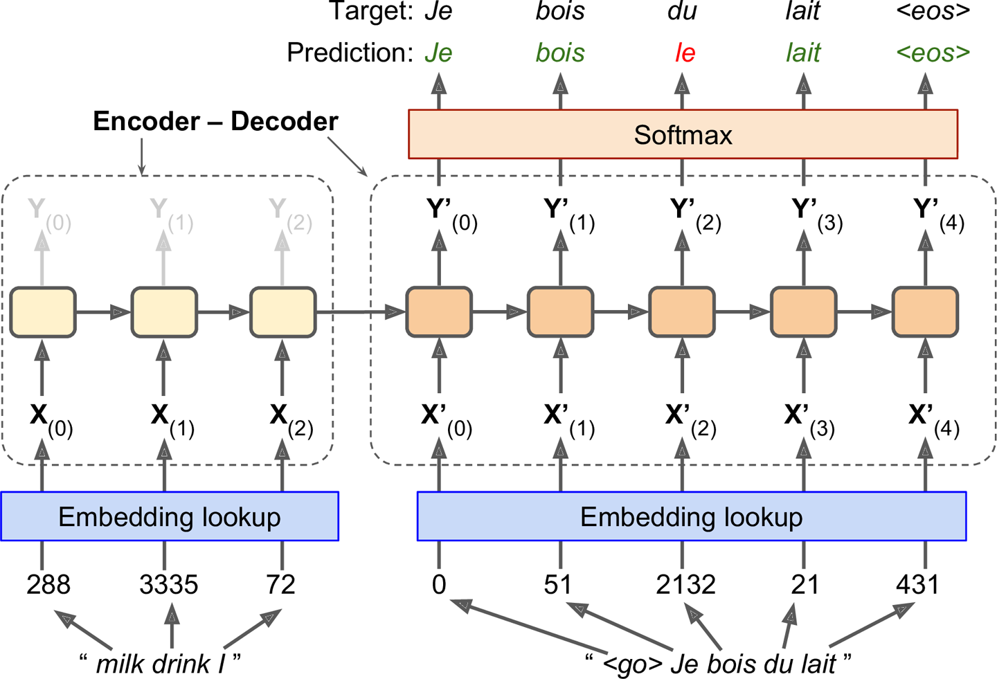
Figure 4-15. A simple machine translation model

The English sentences are fed to the encoder, and the decoder outputs the French translations. Note that the French translations are also used as inputs to the decoder, but pushed back by one step. In other words, the decoder is given as input the word that it should have output at the previous step (regardless of what it actually output). For the very first word, it is given a token that represents the beginning of the sentence (e.g., “<go>”). The decoder is expected to end the sentence with an end-of-sequence (EOS) token (e.g., “<eos>”).

Note that the English sentences are reversed before they are fed to the encoder. For example “I drink milk” is reversed to “milk drink I.” This ensures that the beginning of the English sentence will be fed last to the encoder, which is useful because that’s generally the first thing that the decoder needs to translate.

Each word is initially represented by a simple integer identifier (e.g., 288 for the word “milk”). Next, an embedding lookup returns the word embedding (as explained earlier, this is a dense, fairly low-dimensional vector). These word embeddings are what is actually fed to the encoder and the decoder.

At each step, the decoder outputs a score for each word in the output vocabulary (i.e., French), and then the Softmax layer turns these scores into probabilities. For example, at the first step the word “Je” may have a probability of 20%, “Tu” may have a probability of 1%, and so on. The word with the highest probability is output. This is very much like a regular classification task, so you can train the model using the softmax_cross_entropy_with_logits() function.

Note that at inference time (after training), you will not have the target sentence to feed to the decoder. Instead, simply feed the decoder the word that it output at the previous step, as shown in Figure 4-16 (this will require an embedding lookup that is not shown on the diagram).

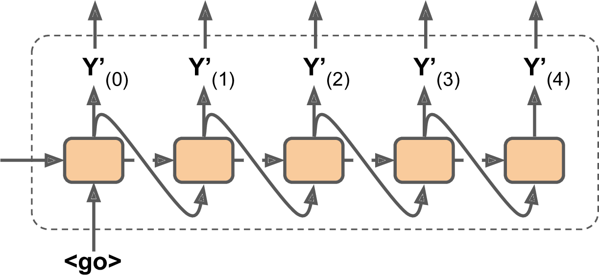
Figure 4-16. Feeding the previous output word as input at inference time

Okay, now you have the big picture. However, if you go through TensorFlow’s sequence-to-sequence tutorial and you look at the code in rnn/translate/seq2seq_model.py (in the TensorFlow models), you will notice a few important differences:

• First, so far we have assumed that all input sequences (to the encoder and to the decoder) have a constant length. But obviously sentence lengths may vary. There are several ways that this can be handled—for example, using the sequence_length argument to the static_rnn() or dynamic_rnn() functions to specify each sentence’s length (as discussed earlier). However, another approach is used in the tutorial (presumably for performance reasons): sentences are grouped into buckets of similar lengths (e.g., a bucket for the 1- to 6-word sentences, another for the 7- to 12-word sentences, and so on¹¹), and the shorter sentences are padded using a special padding token (e.g., “<pad>”). For example “I drink milk” becomes “<pad> <pad> <pad> milk drink I”, and its translation becomes “Je bois du lait <eos> <pad>”. Of course, we want to ignore any output past the EOS token. For this, the tutorial’s implementation uses a target_weights vector. For example, for the target sentence “Je bois du lait <eos> <pad>”, the weights would be set to [1.0, 1.0, 1.0, 1.0, 1.0, 0.0] (notice the weight 0.0 that corresponds to the padding token in the target sentence). Simply multiplying the losses by the target weights will zero out the losses that correspond to words past EOS tokens.

• Second, when the output vocabulary is large (which is the case here), outputting a probability for each and every possible word would be terribly slow. If the target vocabulary contains, say, 50,000 French words, then the decoder would output 50,000-dimensional vectors, and then computing the softmax function over such a large vector would be very computationally intensive. To avoid this, one solution is to let the decoder output much smaller vectors, such as 1,000-dimensional vectors, then use a sampling technique to estimate the loss without having to compute it over every single word in the target vocabulary. This Sampled Softmax technique was introduced in 2015 by Sébastien Jean et al.¹² In TensorFlow you can use the sampled_softmax_loss() function.

• Third, the tutorial’s implementation uses an attention mechanism that lets the decoder peek into the input sequence. Attention augmented RNNs are beyond the scope of this lesson, but if you are interested there are helpful papers about machine translation,¹³ machine reading,¹⁴ and image captions¹⁵ using attention.

• Finally, the tutorial’s implementation makes use of the tf.nn.legacy_seq2seq module, which provides tools to build various Encoder–Decoder models easily. For example, the embedding_rnn_seq2seq() function creates a simple Encoder–Decoder model that automatically takes care of word embeddings for you, just like the one represented in Figure 4-15. This code will likely be updated quickly to use the new tf.nn.seq2seq module.

You now have all the tools you need to understand the sequence-to-sequence tutorial’s implementation. Check it out and train your own English-to-French translator!

Exercises

1. Can you think of a few applications for a sequence-to-sequence RNN? What about a sequence-to-vector RNN? And a vector-to-sequence RNN?

2. Why do people use encoder–decoder RNNs rather than plain sequence-to-sequence RNNs for automatic translation?

3. How could you combine a convolutional neural network with an RNN to classify videos?

4. What are the advantages of building an RNN using dynamic_rnn() rather than static_rnn()?

5. How can you deal with variable-length input sequences? What about variable-length output sequences?

6. What is a common way to distribute training and execution of a deep RNN across multiple GPUs?

7. Embedded Reber grammars were used by Hochreiter and Schmidhuber in their paper about LSTMs. They are artificial grammars that produce strings such as “BPBTSXXVPSEPE.” Check out Jenny Orr’s nice introduction to this topic. Choose a particular embedded Reber grammar (such as the one represented on Jenny Orr’s page), then train an RNN to identify whether a string respects that grammar or not. You will first need to write a function capable of generating a training batch containing about 50% strings that respect the grammar, and 50% that don’t.

8. Tackle the “How much did it rain? II” Kaggle competition. This is a time series prediction task: you are given snapshots of polarimetric radar values and asked to predict the hourly rain gauge total. Luis Andre Dutra e Silva’s interview gives some interesting insights into the techniques he used to reach second place in the competition. In particular, he used an RNN composed of two LSTM layers.

9. Go through TensorFlow’s Word2Vec tutorial to create word embeddings, and then go through the Seq2Seq tutorial to train an English-to-French translation system.

Solutions to these exercises are available in Appendix A.

¹ Note that many researchers prefer to use the hyperbolic tangent (tanh) activation function in RNNs rather than the ReLU activation function. For example, take a look at by Vu Pham et al.’s paper “Dropout Improves Recurrent Neural Networks for Handwriting Recognition”. However, ReLU-based RNNs are also possible, as shown in Quoc V. Le et al.’s paper “A Simple Way to Initialize Recurrent Networks of Rectified Linear Units”.

² This uses the decorator design pattern.

³ “Long Short-Term Memory,” S. Hochreiter and J. Schmidhuber (1997).

⁴ “Long Short-Term Memory Recurrent Neural Network Architectures for Large Scale Acoustic Modeling,” H. Sak et al. (2014).

⁵ “Recurrent Neural Network Regularization,” W. Zaremba et al. (2015).

⁶ “Recurrent Nets that Time and Count,” F. Gers and J. Schmidhuber (2000).

⁷ “Learning Phrase Representations using RNN Encoder–Decoder for Statistical Machine Translation,” K. Cho et al. (2014).

⁸ A 2015 paper by Klaus Greff et al., “LSTM: A Search Space Odyssey,” seems to show that all LSTM variants perform roughly the same.

⁹ For more details, check out Christopher Olah’s great post, or Sebastian Ruder’s series of posts.

¹⁰ “Sequence to Sequence learning with Neural Networks,” I. Sutskever et al. (2014).

¹¹ The bucket sizes used in the tutorial are different.

¹² “On Using Very Large Target Vocabulary for Neural Machine Translation,” S. Jean et al. (2015).

¹³ “Neural Machine Translation by Jointly Learning to Align and Translate,” D. Bahdanau et al. (2014).

¹⁴ “Long Short-Term Memory-Networks for Machine Reading,” J. Cheng (2016).

¹⁵ “Show, Attend and Tell: Neural Image Caption Generation with Visual Attention,” K. Xu et al. (2015).