Online Investing Hacks

Use Rational Values to Buy and Sell Wisely

By determining the rational value of stocks, improve your investment results by keeping emotions out of your buy and sell decisions.

It’s really tough for an investor to remain upbeat and hold investments whose prices are plummeting in the throes of a down market. And it’s equally difficult to be realistic and patient (the cornerstones of successful investing) when the stock market is soaring. By assessing the rational price of a stock and the rational value of your portfolio, you can make sensible choices when others overreact.

Many shareholders fail to realize that there is a finite, absolute—though approximate—value for each share of stock. When viewed over a five-year period, the short-term ups and downs of a stock’s price generally vary on either side of a value that’s tied to the earnings of the underlying company. When you select successful companies capable of growing their earnings at a substantial rate, the underlying value of your shares should climb as well.

The relationship between a company’s earnings and its stock’s price is measured by the price to earnings ratio [Hack #27] and is calculated by dividing the price of a share of the stock by the company’s earnings per share. Called the P/E ratio or multiple, this value is similar to the price per pound of coffee or gallon of gas. The P/E ratio is the price investors are willing to pay for a dollar’s worth of the underlying company’s earnings.

The Signature PE

Because it fluctuates constantly with the price, looking at the P/E ratio at any given moment isn’t going to be that helpful. However, the average of those P/E ratios over a significant period of time can provide a typical, reasonable multiple of earnings to which the P/E ratio returns from higher or lower values, shown in Table 4-10. This value is called the signature PE.

Table 4-10. Using ten years of P/E ratios to identify the signature PE

Year	EPS	High price	Low price	High PE	Low PE
1993	0.39	5.60	4.10	14.4	10.5
1994	0.47	6.00	4.20	12.8	8.9
1995	0.58	7.50	5.30	12.9	9.1
1996	0.68	11.00	7.10	16.2	10.4
1997	1.04	14.50	9.40	13.9	9.0
1998	0.88	22.70	11.30	25.8	12.8
1999	1.04	28.40	19.50	27.3	18.8
2000	1.14	37.50	16.80	32.9	14.7
2001	1.28	36.10	23.00	28.2	18.0
2002	1.55	33.50	23.10	21.6	14.9
Median values				18.9	11.7
Average or signature PE					15.3

Until the end of the twentieth century, looking at the average P/E ratio over a five-year period seemed adequate because the average economic or business cycle ran its course in that length of time. However, the duration and amplitude of the most recent boom and ensuing bust have shown that we must consider an average P/E ratio over a longer period of time.

To arrive at a signature PE, the best approach is to calculate the high and low P/E ratios for the last ten years, calculate their medians to eliminate anomalous data above and below, then average the resulting values. Unlike an average, the median is the value with equal numbers of entries above and below. If there is an even number of values, the median is the average of the two middle values of the set of numbers.

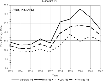
Table 4-10 shows the calculation for the signature PE using the high and low prices and the earnings data for Aflac Inc. (AFL), the insurance company. When you consider that the signature PE represents a reasonable rate to pay for a dollar’s worth of Aflac’s earnings, it’s easy to see in Table 4-10 that there were times—indeed entire years—when investors paid more than a reasonable P/E ratio and times when they paid less. By its definition, the average multiple paid for this stock was above the signature PE about half the time and below it the other half.

When the current P/E ratio is above the signature PE, the P/E ratio is likely to eventually decline; if the P/E ratio is below, it should sooner or later grow. Looking at the chart in Figure 4-24, you can see that, although the amplitude of the swing above or below might vary, the P/E ratios rise or fall to gravitate toward the signature PE.

Figure 4-24. The P/E ratio varies above and below the signature PE

The Historical Value Ratio

How can you put the P/E ratio’s tendency to return to the signature PE to practical use? There are several ways. When contemplating the purchase of a stock, look at the current P/E ratio and compare it to the signature PE. If the current P/E ratio is much above the signature PE, the stock is probably too pricey and will likely go down over time. If it’s below, you might have a bargain.

Tip

Before you snap up what looks like a bargain, you should question what others might know about the company that you don’t. Something might be causing folks to sell and pushing the price below where it’s traditionally been.

Dividing the current P/E ratio by the signature PE produces the historical value ratio (HVR). This is a way to quantify the comparison. If the HVR is more than, say, 110 percent, the rate for a dollar’s worth of earnings is more than 10 percent above the typical rate. You probably should wait for the price to fall into a more reasonable range. If your HVR is below 90 percent, be careful. There might be a very good reason.

Rational Price and Rational Value

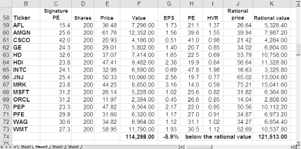
Probably the most useful purpose for the HVR is the calculation of a rational price and its derivative, rational value. The rational price of a stock is simply the price you would pay if the stock were selling at its signature PE, i.e., an HVR of 100 percent. If you’ve calculated the HVR for a stock, you can figure out the rational price by simply dividing the current price by the HVR. When the HVR is below 100 percent, the rational price for a stock is higher than the current price. When the HVR is elevated, the rational price is lower than the current price.

From this, it’s easy to see that the rational value of your holdings in that company would be the product of the rational price and the number of shares you own. And the rational value of your portfolio would be the sum of the rational values of the stocks within it.

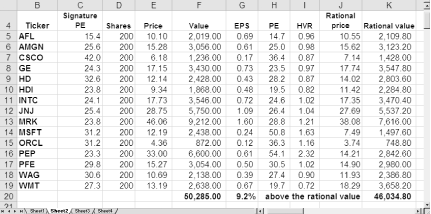
Relative value [Hack #27] is similar to rational value but utilizes the average P/E ratio of the most recent five years in lieu of the median over ten years. Looking at the chart in Figure 4-25, the elevated P/E ratios of the most recent five years show why using ten years of P/E ratio data is preferable. It would produce a more rational result than the more optimistic values of the past five years. However, you can use relative value as a quick-and-dirty method of arriving at the rational value. If you choose to use relative value, you must do your utmost to eliminate irrelevant, anomalous data from the five-year history before dividing the current price by the relative value to produce the rational price.

To see the benefit of using rational value to evaluate a portfolio, let’s view a sample portfolio of 15 of the most widely held stocks at different points during the most recent bull and bear markets.

Figure 4-25. Prices were just over their rational value in February 1997

Figure 4-25 shows that prices were relatively normal in February of 1997, priced a bit above the rational value. Investors were becoming a bit exuberant. If stocks were selling at a P/E ratio about what they had historically sold for, the portfolio’s value would have been around $46,000, but investors were willing to pay $50,285.

Tip

Earnings and prices have been adjusted to compensate for splits.

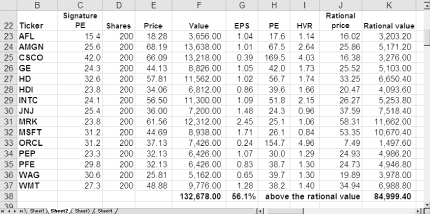
In February of 2000, optimism was in full swing, near the peak of the period of irrational exuberance when the Greater Fool Theory dominated the decision making process. The market valued this portfolio at more than $132,000—more than 56 percent above the rational prices for its stocks, as shown in Figure 4-26. The increase in rational value from February 1997 was a natural result of earnings growth. The P/E ratios above the signature PEs as well as HVR values higher than 1.0 were telltale signs that the market was seriously inflated. Calculating the rational value is a good way to keep your feet on the ground in times like these.

Figure 4-26. In February 2000, investors were paying irrationally high prices for stocks

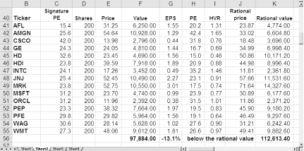
By February of 2003 the bubble had burst, and the value of the portfolio, measured by what the now irrationally fearful market was paying for good quality stocks, had plummeted 27 percent from its high. Investors who had been willing to pay $132,000 for a portfolio rationally worth $84,999 were now paying only $97,884 for stocks rationally worth $112,613, as shown in Figure 4-27. The rational value of this portfolio, based on earnings growth, had continued to increase, even while those who didn’t know any better were practically giving away their stocks. In times like these, when the hardiest of the long-term investors are suffering doubts and fears, it’s helpful to look at the rational value to realize that the actual value of the portfolio should be considerably higher—and will be just as soon as the market comes back to its senses and pays a reasonable multiple of earnings for the stocks.

Figure 4-27. In February 2003, investors reversed themselves and were paying less than stocks were worth

Sure enough, only eight months from the depths of the market collapse, the market value of the portfolio had already exceeded the rational value from the previous February, as shown in Figure 4-28. What’s more, the rational value had increased with the healthy increases in earnings that attended the end of the recession. This portfolio still has plenty of P/E ratio expansion to enjoy as its market value climbs to reach its current rational value.

Figure 4-28. A recent look at the rational value of several stocks

Code

One of the best sources of data for this exercise [Hack #20] is NAIC’s .ssg files, available through NAIC (Online Premium Service), or data available through AAII’s Stock Investor Pro. When you open an .ssg file for any stock in Excel, the entire file is stored in column A, cells 1 through 531. You can set up an Excel template for these files using a defined array variable to calculate the HVR for a company.

Files in .ssg format contain the data you need in the following cells:

Annual high prices = $A$1:$A$10

Annual low prices = $A$11:$A$20

Annual earnings per share = $A$71:$A$80

Current PE = $A$92

To create named ranges [Hack #9] in your Excel file, select the cells you want to add to a named range and choose Insert Name→Define. Type the name for the range in the Names In Workbook box and click Add.

Name and define the ranges in Table 4-11 if you use .ssg files for data. If you use a different data source, substitute these cell ranges with the cell ranges for the same data in your data source.

Table 4-11. Named ranges for calculating rational values

Named range	Cell range
HighPrices	$A$1:$A$10
LowPrices	$A$11:$A$20
EPS	$A$71:$A$80
PE	$A$92
HVR	$D$1

To calculate HVR, type the formula in Example 4-51 in the HVR cell, and then create an array formula by pressing Shift-Ctrl-Enter.

Example 4-51. Formula for calculating the HVR

HVR = PE / (AVERAGE(MEDIAN(IF(HighPrices<>0,HighPrices/EPS)),
    MEDIAN(IF(LowPrices<>0,LowPrices/EPS))))

The IF function evaluates empty cells as zero. However, the formula in Example 4-51 won’t generate a divide by zero error for companies with less than 10 years of data. The third argument for the IF function is missing as well as the comma preceding the third argument. This means that when a value in the HighPrices or LowPrices named range equals zero, the IF function returns False, which in turn triggers the MEDIAN function to ignore that data point because it’s text. If you were to include the comma in the IF function, the formula would generate a divide by zero error.

Tip

An array formula permits arrays to be manipulated mathematically by other arrays. When you type an array formula in a worksheet cell, Excel places brackets ({}) around the formula, which appear in the formula bar when you select the cell.

To display the value for HVR in a cell in the worksheet, type =HVR in the cell. Because named ranges apply to an entire workbook, you can type =HVR in any cell in any worksheet within the Excel workbook. This formula returns the HVR of the company using as many years of P/E ratio history as are available.

—Ellis Traub