Practical Automated Machine Learning on Azure

Chapter 4. Feature Engineering and Automated Machine Learning

Feature engineering is one of the most important parts of the data science process. If you ask data scientists to break down the time spent in each stage of the data science process, you’ll often hear that they spend a significant amount of time understanding and exploring the data, and doing feature engineering. Most experienced data scientists do not jump into model building. Rather, they first spend time doing feature engineering.

But what is feature engineering? With feature engineering, you can transform your original data into a form that is more easily understood by the machine learning algorithms. For example, you might perform data processing, add new features (e.g., additional data columns that combine values from existing columns), or you might transform the features from their original domain to a different domain. You might also remove features that are not useful or relevant to the model. When doing feature engineering, you will generate new features, transform existing features, or select a subset of features.

To illustrate how you can transform features, let’s consider a simple example of working with categorical features (otherwise known as categorical variables). Suppose that you have a dataset for an airline customer program with a feature called Status, which determines the status of the customers (e.g., based on how often the customer flies, total miles traveled, and others). Status contains the following five unique values: New, Silver, Gold, Platinum, and Diamond. Because some of the machine learning algorithms can work only with numerical variables, you will need to transform the feature. A common approach is to use one-hot encoding, as shown in Table 4-1.

Table 4-1. One-hot encoding

Status		New	Silver	Gold	Platinum	Diamond
Gold		0	0	1	0	0
Silver		0	1	0	0	0
New	➪	1	0	0	0	0
Platinum		0	0	0	1	0
Silver		0	1	0	0	0
Gold		0	0	1	0	0

Another important aspect of feature engineering is taking advantage of domain expertise. You might consider working with a person who has relevant domain expertise when doing feature engineering—the inputs from the domain expert will be invaluable when working toward the goal of delivering a high-quality model.

Transparency and explainability are important considerations when training machine learning models. Hence, doing feature engineering properly will contribute toward having high-performing models that can be explained.

Note

Chapter 7 provides a detailed discussion on how Azure Machine Learning gives you the tools to understand the models generated, the relative importance of features, and more.

When performing feature engineering, data scientists often ask themselves the following questions:

• Which features in the dataset are irrelevant to the model? For example, your data might contain an Identifier (ID) column. Though this column is useful when combining data from several datasets (e.g., joining two datasets based on an employee_id), the ID column is not used in any way when training the model.

• Can we combine one or more features to create new features that will be even more useful?

• For some of the classes that are sparse (i.e., those that contain significantly fewer observations), can we group them to create more meaningful classes?

In this chapter, we focus on how to use the auto-featurization capabilities provided in the automated ML tool that is a part of Microsoft Azure Machine Learning. You will learn how auto-featurization works for classification, regression, and forecasting tasks. In addition, we share pointers and resources that enable you to go more in-depth with feature engineering. Before we dive into the auto-featurization performed by automated ML, let’s look at the data preprocessing methods that are available.

Data Preprocessing Methods Available in Automated ML

Depending on the type of machine learning task (e.g., classification, regression, forecasting), different types of data preprocessing are performed. When you use automated ML and submit an experiment, you will notice that each iteration performs a different type of data preprocessing.

For example, you will notice that your data is scaled, or normalized, when it is relevant. When features have different ranges, scaling and normalization helps. Table 4-2 shows the scaling and normalization steps performed by automated ML.

Table 4-2. Data preprocessing performed by automated ML

Scaling and normalization	Description
MinMaxScalar	Each feature is transformed by scaling to the minimum and maximum for that column.
MaxAbsScaler	Each feature is scaled by using the maximum absolute value.
RobustScalar	Each feature is scaled by using the values from quantile range.
PCA	Linear dimensionality reduction using singular value decomposition (SVD) of the data to project it to a lower dimensional space.
TruncatedSVDWrapper	Uses truncated SVD to do linear dimensionality reduction. Unlike principal component analysis (PCA), the data is not centered before SVD is computed. Note: This enables it to work efficiently with scipy.sparse matrices.
SparseNormalizer	Each sample that contains one or more nonzero components is independently rescaled, enabling the norm (L1 or L2) to equal one.

Tip

For more details on how data is preprocessed in Azure Machine Learning, see this section of the Microsoft Azure documentation.

Auto-Featurization for Automated ML

Let’s get started with using auto-featurization. By now, you should be familiar with how to set up the automated ML configuration object. Let’s recap how you set up the automated ML experiment. In the code example that follows, you first define the AutoMLConfig object. Next, specify the name of the experiment, number of iterations to run, the logging granularity, and more. After you have defined the AutoMLConfig object, submit the experiment by using experiment.submit(…):

import time

automl_settings = {
    "name": "AutoML_Book_CH07_FeatureEngineering_{0}".format(time.time()),
    "task": "regression",
    "iteration_timeout_minutes": 10,
    "iterations": 10,
    "max_cores_per_iteration": 1,
    "primary_metric": 'r2_score',
    "max_concurrent_iterations": 10,
    "experiment_exit_score": 0.985,
    "debug_log": "automl_ch07_errors{0}.log".format(time.time()),
    "verbosity": logging.ERROR
}
# Local compute
Automl_config = AutoMLConfig(
                   preprocess = False,
                   X = X_train,
                   y = y_train,
                   X_valid = X_valid,
                   y_valid = y_valid,
                   path=project_folder,
                   **automl_settings)

# Training the model
experiment=Experiment(ws, experiment_name)
local_run = experiment.submit(Automl_config, show_output=True)

After you submit the experiment, notice the data processing that has been performed in each iteration (see the output in Figure 4-1). From iteration 0 to 7, you can see that each iteration shows what type of data preprocessing has been performed. For example, in iteration 0, we can see that the StandardScalerWrapper is used. In iteration 3, the RobustScaler is used.

In the code shown earlier, in which you defined the AutoMLConfig object, notice that one of the properties, preprocess, is set to False. You can also set preprocess = True to turn on advanced data preprocessing. This makes it possible for you to use both data preprocessing and auto-featurization.

Note

The type of auto-featurization performed depends on the machine learning task you’re planning. For example, if you use automated ML for classification and regression, auto-featurization might include dropping features with a high cardinality, or low variance. If you use automated ML for forecasting, additional features might be generated for DateTime, or relation of the DateTime to holidays in various countries.

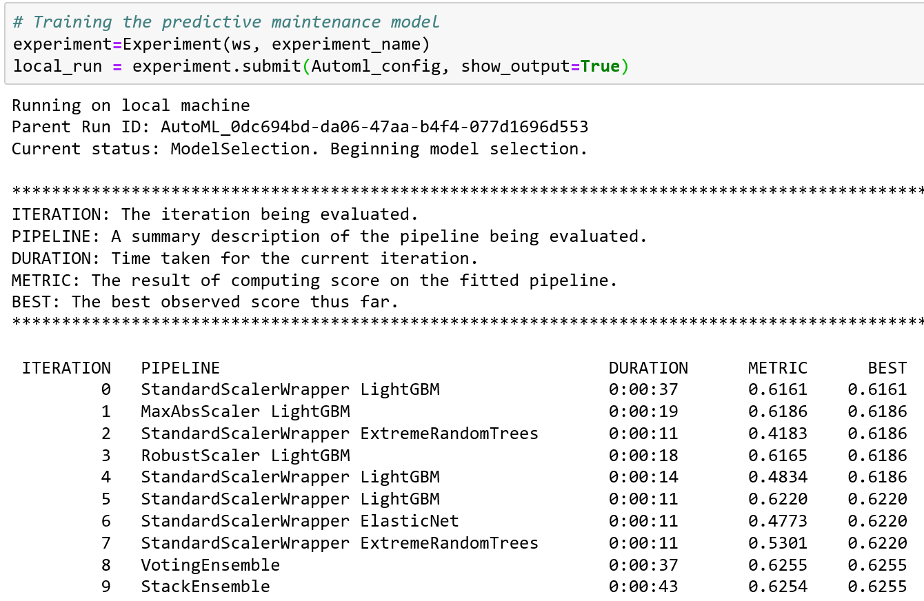
Figure 4-1. Data preprocessing using automated ML

Table 4-3 presents the auto-featurization features used by automated ML.

Table 4-3. Auto-featurization performed by automated ML

Preprocessing and auto-featurization	Description
Drop high-cardinality or no variance features	Drop these from training and validation sets, including features with all values missing, same value across all rows, or with extremely high-cardinality (e.g., hashes, IDs, or GUIDs).
Impute missing values	For numerical features, impute with average of values in the column. For categorical features, impute with most frequent value.
Generate additional features	For DateTime features: Year, Month, Day, Day of week, Day of year, Quarter, Week of the year, Hour, Minute, Second. For Text features: Term frequency based on unigrams, bi-grams, and tri-character-grams.
Transform and encode	Numeric features with few unique values are transformed into categorical features. One-hot encoding is performed for low cardinality categorical; for high cardinality, one-hot-hash encoding.
Word embeddings	Text featurizer that converts vectors of text tokens into sentence vectors using a pretrained model. In a given document, each word’s embedding vector is aggregated to produce a document feature vector.
Target encodings	For categorical features, maps each category to averaged target value for regression problems. For classification problems, maps each category to the class probability for each class. Frequency-based weighting and k-fold cross-validation is applied to reduce overfitting of the mapping and noise caused by sparse data categories.
Text target encoding	For text input, a stacked linear model with bag-of-words is used to generate the probability of each class.
Weight of Evidence (WoE)	Calculates WoE as a measure of correlation of categorical columns to the target column. It is calculated as the log of the ratio of in-class versus out-of-class probabilities. This step outputs one numerical feature column per class and removes the need to explicitly impute missing values and outlier treatment.
Cluster distance	Trains a k-means clustering model on all numerical columns. Outputs k new features, one new numerical feature per cluster, containing the distance of each sample to the centroid of each cluster.

Auto-Featurization for Classification and Regression

To show auto-featurization in action, let’s work through a predictive maintenance model using the NASA Turbofan Engine Degradation Simulation dataset. In this example, even though we show how regression is used to predict the remaining useful lifetime (RUL) value for the turbofan engine, we can apply the same approach to classification problems as well.

To do this, let’s first download the dataset using the code block that follows. After you download the dataset, you extract the file into the data folder, and read the training data file, data/train_FD004.txt. Then, you add the column names for the 26 features. Use the following code to do this:

# Download the NASA Turbofan Engine Degradation Simulation Dataset
import requests, zipfile, io
import pandas as pd
nasa_dataset_url = https://ti.arc.nasa.gov/c/6/
r = requests.get(nasa_dataset_url)

z = zipfile.ZipFile(io.BytesIO(r.content))
z.extractall("data/")
train = pd.read_csv("data/train_FD004.txt", delimiter="\s|\s\s",
          index_col=False, engine='python',
          names=['unit','cycle','os1','os2','os3',
                 'sm1','sm2','sm3','sm4','sm5','sm6','sm7','sm8',
                 'sm9','sm10', 'sm11','sm12','sm13','sm14','sm15','sm16',
                 'sm17','sm18','sm19','sm20','sm21'])

An important part of the data science process is to explore the dataset. Since we use this dataset in other chapters, we won’t explore it here. In addition, we’ll omit the steps needed to create the Azure Machine Learning experiment and set up the AutoMLConfig object (shown earlier) and proceed directly to exploring the differences and quality of results when preprocess is set to different values (i.e., True or False).

Before we do that, let’s define the utility functions that will be useful in the exploration. We will create two utility functions: print_model() (Example 4-1), and print_engineered_features() (Example 4-2). These two utility functions are used to print the pipelines for a model, and the features that are generated during auto-featurization, respectively, as shown in the following examples.

Example 4-1. print_model

from pprint import pprint

def print_model(run, model, prefix=""):
    print(run)
    print("---------")

for step in model.steps:
    print(prefix + step[0])
    if hasattr(step[1], 'estimators') and hasattr(step[1], 'weights'):
         pprint({'estimators': list(e[0] for e in step[1].estimators),
             'weights': step[1].weights})

         print()
         for estimator in step[1].estimators:
            print_model(estimator[1], estimator[0]+ ' - ')
    elif hasattr(step[1], '_base_learners') and
         hasattr(step[1], '_meta_learner'):

         print("\nMeta Learner")
         pprint(step[1]._meta_learner)
         print()

         for estimator in step[1]._base_learners:
            print_model(estimator[1], estimator[0]+ ' - ')
    else:
        pprint(step[1].get_params())
        print()

Example 4-2. print_engineered_features

from pprint import pprint
import pandas as pd
# Function to pretty print the engineered features
def print_engineered_features(features_summary):
    print(pd.DataFrame(features_summary,
          columns=["RawFeatureName",
                   "TypeDetected",
                   "Dropped",
                   "EngineeredFeatureCount",
                   "Tranformations"]))

Now that we have defined the two utility functions, let’s explore two iterations for an experiment in which preprocess is set to False, and the data preprocessing shown in the outputs are similar. (Figure 4-1 shows the output after the experiment is submitted.) Iterations 4 and 5 of the experiment use the same data processing technique (StandardScalerWrapper) and the same machine learning algorithm (LightGBM). What’s the difference between the two iterations, and why do they show two different R2 score values? Iteration 5 (R2 score of 0.6220) seems to have performed better than iteration 4 (R2 score of 0.4834).

Using local_run.get_output(), we extracted the run and models that have been trained for iterations 4 and 5. The run information is stored in explore_run1 and explore_run2, and the model details are stored in explore_model1 and explore_model2:

explore_run1, explore_model1 = local_run.get_output(iteration = 4)
explore_run2, explore_model2 = local_run.get_output(iteration = 5)

After you have extracted the run information and model details, let’s look at them closely. From the output for iterations 4 and 5 shown, you will notice the hyperparameter values are different (e.g., max_bin, max_depth, learning_rate, reg_alpha, reg_lambda, and others). These hyperparameter values are determined by the automated ML meta-model that has been trained to decide which machine learning pipeline will be most relevant to the dataset (see Examples 4-3 and 4-4.

Note

See Chapter 2 for more on how Automated Machine Learning works.

Example 4-3. Iteration 4 run and model information

Run(Experiment: automl-predictive-rul-ch07,
Id: AutoML_0dc694bd-da06-47aa-b4f4-077d1696d553_4,
Type: None,
Status: Completed)
---
StandardScalerWrapper
{'class_name': 'StandardScaler',
 'copy': True,
 'module_name': 'sklearn.preprocessing.data',
 'with_mean': False,
 'with_std': True}

LightGBMRegressor
{'boosting_type': 'gbdt',
 'class_weight': None,
 'colsample_bytree': 0.7000000000000001,
 'importance_type': 'split',
 'learning_rate': 0.1894742105263158,
 'max_bin': 7,
 'max_depth': 3,
 'min_child_samples': 139,
 'min_child_weight': 0.001,
 'min_split_gain': 0.9473684210526315,
 'n_estimators': 800,
 'n_jobs': 1,
 'num_leaves': 7,
 'objective': None,
 'random_state': None,
 'reg_alpha': 0.075,
 'reg_lambda': 0.6,
 'silent': True,
 'subsample': 0.7999999999999999,
 'subsample_for_bin': 200000,
 'subsample_freq': 0,
 'verbose': −1}

Example 4-4. Iteration 5 run and model information

Run(Experiment: automl-predictive-rul-ch07,
Id: AutoML_0dc694bd-da06-47aa-b4f4-077d1696d553_5,
Type: None,
Status: Completed)
---
StandardScalerWrapper
{'class_name': 'StandardScaler',
 'copy': True,
 'module_name': 'sklearn.preprocessing.data',
 'with_mean': True,
 'with_std': True}

LightGBMRegressor
{'boosting_type': 'gbdt',
 'class_weight': None,
 'colsample_bytree': 0.5,
 'importance_type': 'split',
 'learning_rate': 0.1789484210526316,
 'max_bin': 255,
 'max_depth': 9,
 'min_child_samples': 194,
 'min_child_weight': 0.001,
 'min_split_gain': 0.9473684210526315,
 'n_estimators': 100,
 'n_jobs': 1,
 'num_leaves': 127,
 'objective': None,
 'random_state': None,
 'reg_alpha': 1.125,
 'reg_lambda': 0.75,
 'silent': True,
 'subsample': 0.7,
 'subsample_for_bin': 200000,
 'subsample_freq': 0,
 'verbose': −1}

Next, let’s look at the names of the engineered features. To do this, you can use the function get_engineered_feature_names (). The code shows how you retrieve the best run and model by using local_run.get_output() and then extract the names of the engineered features:

best_run, fitted_model = local_run.get_output()
fitted_model.named_steps['datatransformer']. get_engineered_feature_names ()

Figure 4-2 shows the output. In this example, you will see that the engineered features are derived from using the MeanImputer transform on the existing features. No additional features have been added.

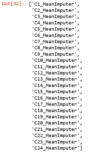
Figure 4-2. Names of engineered features

Let’s dive deeper and look at more details about the engineered features. To do this, use the get_featurization_summary() function. The utility function print_engineered_features() that we defined earlier will enable us to pretty-print the output and make it easier to read.

Figure 4-3 shows the summary of the engineered features. For each original feature, you will see that the MeanImputer transform is applied to it and that the count for new engineered features is 1. You will also observe that no features were dropped when data preprocessing and auto-featurization are performed:

# Get the summary of the engineered features
features_summary =
   fitted_model.named_steps['datatransformer'].get_featurization_summary()
print_engineered_features(features_summary)

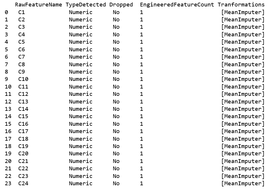
Figure 4-3. Summary of engineered features

Auto-Featurization for Time-Series Forecasting

In this next example, we show how data preprocessing and auto-featurization is performed for a time-series dataset, in which the data type for some of the features is DateTime.

Let’s begin by downloading the sample Energy Demand dataset (Figure 4-4 shows the output from running the code):

import requests, zipfile, io

# Download the data for energy demand forecasting

nyc_energy_data_url =
"https://raw.githubusercontent.com/Azure/MachineLearningNotebooks/master/
          how-to-use-azureml/automated-machine-learning/
          forecasting-energy-demand/nyc_energy.csv"

r = requests.get(nyc_energy_data_url)
open('data/nyc_energy.csv', 'wb').write(r.content)

data = pd.read_csv('data/nyc_energy.csv', parse_dates=['timeStamp'])
data.head()

In Figure 4-4, you can see that the Energy Demand time-series dataset consists of these five columns: ID (leftmost column), timestamp, demand, precip, and temp.

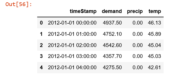
Figure 4-4. Exploring the Energy Demand time-series dataset

Let’s do a simple plot of the data by using the following code (Figure 4-5 shows the output):

import matplotlib.pyplot as plt

time_column_name = 'timeStamp'
target_column_name = 'demand'

ax = plt.gca()
data.plot(kind='line',x=time_column_name,y=target_column_name,ax=ax)
plt.show()

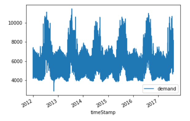
Figure 4-5. Visualization of the Energy Demand time-series dataset

Next, let’s split the data into training and testing datasets, into observations before 2017-02-01 (training dataset), and observations after 2017-02-01 (testing dataset). We extract the target column (the column for the demand values) into y_train and y_test:

X_train = data[data[time_column_name] < '2017-02-01']
X_test = data[data[time_column_name] >= '2017-02-01']
y_train = X_train.pop(target_column_name).values
y_test = X_test.pop(target_column_name).values

Let’s specify the automated ML configuration that we will use for forecasting. In the code that follows, notice that we specify the evaluation metrics for the AutoMLConfig object as the normalized root-mean-square error (RMSE). We also specify the DateTime column using time_column_name.

As each row of the data denotes hourly observations, it is important to specify the time horizon for prediction by using the property max_horizon. Suppose that you want to predict for the next one day (i.e., 24 hours); the value of max_horizon is set to 24. The property country_or_region is commented out in this example. This property is useful if you want to take into consideration autogenerated features that capture details about the holidays in the country specified. In this specific example, we do not need it; thus, we comment it out:

time_series_settings = {
    "time_column_name": time_column_name,
    "max_horizon": 24
    #"country_or_region" : 'US',
}

automl_config = AutoMLConfig(task = 'forecasting',
                   primary_metric='normalized_root_mean_squared_error',
                   iterations = 10,
                   iteration_timeout_minutes = 5,
                   X = X_train,
                   y = y_train,
                   n_cross_validations = 3,
                   path=project_folder,
                   verbosity = logging.INFO,
                   **time_series_settings)

Now that you have defined the AutoMLConfig object, you are ready to submit the experiment. Figure 4-6 presents the output of running the experiment. When the automated ML experiment is run, you will see that the experiment starts by performing auto-featurization on the time-series dataset. This is captured in the steps “Current status: DatasetFeaturization. Beginning to featurize the dataset.” and “Current status: DatasetFeaturizationCompleted. Completed featurizing the dataset.” After featurization is completed, model selection using automated ML begins.

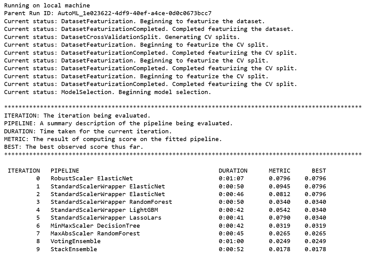
Figure 4-6. Running the automated ML experiment

During model selection, automated ML runs several iterations. Each iteration uses different data preprocessing methods (e.g., RobustScaler, StandardScalerWrapper, MinMaxScaler, MaxAbsScaler) and forecasting algorithms (ElasticNet, LightGB, LassoLars, DecisionTree, and RandomForest). The last two iterations use different ensemble methods (e.g., VotingEnsemble and StackEnsemble). For this specific example, the best result is achieved in iteration 9, which uses StackEnsemble:

local_run = experiment.submit(automl_config, show_output=True)

Now, let’s retrieve detailed information about the best run and the model. Figure 4-7 shows the summary of the engineered features. As this is a time-series dataset, you’ll notice that for the feature timestamp, 11 additional features are autogenerated (i.e., EngineeredFeatureCount is shown as 11), all of data type DateTime.

best_run, fitted_model = local_run.get_output()

# Get the summary of the engineered features
fitted_model.named_steps['timeseriestransformer'].get_featurization_summary()

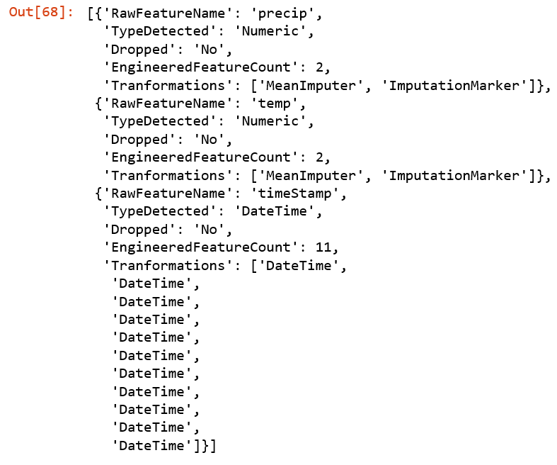
Figure 4-7. Retrieving information for the best run

Let’s now examine the features autogenerated for the DateTime column. To do this, we’ll use fitted_model for performing forecasting, using the test data we defined earlier. From the following code, we invoke the forecast function, and the results are stored in the variables y_fcst and X_trans:

best_run, fitted_model = local_run.get_output()

y_query = y_test.copy().astype(np.float)
y_query.fill(np.NaN)
y_fcst, X_trans = fitted_model.forecast(X_test, y_query)

Next we turn to X_trans. In Figure 4-8, you can see the 11 engineered features, which took the DateTime column and divided it into the time parts (e.g., year, half, quarter, month, day, hour, am_pm, hour12, wday, qday, and week). Changing it from a DateTime to a numerical value makes it more meaningful and easier to use by the machine learning algorithms during training and scoring.

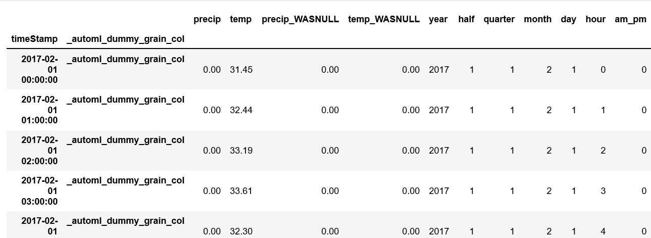
Figure 4-8. Engineered features for time-series forecasting

Conclusion

In this chapter, you learned about the importance of feature engineering, and how it affects the quality of the machine learning models produced. Feature engineering is an art: to do it well, it’s important to understand its foundations, to receive on-the-job training, and to build your toolbox for doing feature engineering as you work through various machine learning projects. In recent years, the machine learning community has been innovating on Python libraries that enable auto-featurization. For example, you can use the Python package featuretools to perform deep feature synthesis by taking advantage of the relationships between entities, and more.

We focused in this chapter on how to use the auto-featurization capabilities provided by automated ML in the Azure Machine Learning service. Using examples of regression and forecasting, we explored how to enable auto-featurization in automated ML and how to understand the engineered features.

Though automated ML provides auto-featurization capabilities (that are continuously improving and evolving), note that it doesn’t exhaustively cover all aspects of feature engineering. It’s important for data scientists to perform feature engineering, taking advantage of domain expertise, before using the dataset as input to automated ML.