Chapter 4. Text Classification
Organizing is what you do before you do something,
so that when you do it, it is not all mixed up.A.A. Milne
All of us check email every day, possibly multiple times. A useful feature of most email service providers is the ability to automatically segregate spam emails away from regular emails. This is a use case of a popular NLP task known as text classification, which is the focus of this chapter. Text classification is the task of assigning one or more categories to a given piece of text from a larger set of possible categories. In the email spam–identifier example, we have two categories—spam and non-spam—and each incoming email is assigned to one of these categories. This task of categorizing texts based on some properties has a wide range of applications across diverse domains, such as social media, e-commerce, healthcare, law, and marketing, to name a few. Even though the purpose and application of text classification may vary from domain to domain, the underlying abstract problem remains the same. This invariance of the core problem and its applications in a myriad of domains makes text classification by far the most widely used NLP task in industry and the most researched in academia. In this chapter, we’ll discuss the usefulness of text classification and how to build text classifiers for our use cases, along with some practical tips for real-world scenarios.
In machine learning, classification is the problem of categorizing a data instance into one or more known classes. The data point can be originally of different formats, such as text, speech, image, or numeric. Text classification is a special instance of the classification problem, where the input data point(s) is text and the goal is to categorize the piece of text into one or more buckets (called a class) from a set of pre-defined buckets (classes). The “text” can be of arbitrary length: a character, a word, a sentence, a paragraph, or a full document. Consider a scenario where we want to classify all customer reviews for a product into three categories: positive, negative, and neutral. The challenge of text classification is to “learn” this categorization from a collection of examples for each of these categories and predict the categories for new, unseen products and new customer reviews. This categorization need not always result in a single category, though, and there can be any number of categories available. Let’s take a quick look at the taxonomy of text classification to understand this.
Any supervised classification approach, including text classification, can be further distinguished into three types based on the number of categories involved: binary, multiclass, and multilabel classification. If the number of classes is two, it’s called binary classification. If the number of classes is more than two, it’s referred to as multiclass classification. Thus, classifying an email as spam or not-spam is an example of binary classification setting. Classifying the sentiment of a customer review as negative, neutral, or positive is an example of multiclass classification. In both binary and multiclass settings, each document belongs to exactly one class from C, where C is the set of all possible classes. In multilabel classification, a document can have one or more labels/classes attached to it. For example, a news article on a soccer match may belong to more than one category, such as “sports” and “soccer,” simultaneously, whereas another news article on US elections may have the labels “politics,” “USA,” and “elections.” Thus, each document has labels that are a subset of C. Each article can be in no class, exactly one class, multiple classes, or all of the classes. Sometimes, the number of labels in the set C can be very large (known as “extreme classification”). In some other scenarios, we may have a hierarchical classification system, which may result in each text getting different labels at different levels in the hierarchy. In this chapter, we’ll focus only on binary and multiclass classification, as those are the most common use cases of text classification in the industry.
Text classification is sometimes also referred to as topic classification, text categorization, or document categorization. For the rest of this book, we’ll stick to the term “text classification.” Note that topic classification is different from topic detection, which refers to the problem of uncovering or extracting “topics” from texts, which we’ll study in Chapter 7.
In this chapter, we’ll take a closer look at text classification and build text classifiers using different approaches. Our aim is to provide an overview of some of the most commonly applied techniques along with practical advice on handling different scenarios and decisions that have to be made when building text classification systems in practice. We’ll start by introducing some common applications of text classification, then we’ll discuss what an NLP pipeline for text classification looks like and illustrate the use of this pipeline to train and test text classifiers using different approaches, ranging from the traditional methods to the state of the art. We’ll then tackle the problem of training data collection/sparsity and different methods to handle it. We’ll end the chapter by summarizing what we learned in all these sections along with some practical advice and a case study.
Note that, in this chapter, we’ll only deal with the aspect of training and evaluating the text classifiers. Issues related to deploying NLP systems in general and performing quality assurance will be discussed in Chapter 11.
Applications
Text classification has been of interest in a number of application scenarios, ranging from identifying the author of an unknown text in the 1800s to the efforts of USPS in the 1960s to perform optical character recognition on addresses and zip codes [1]. In the 1990s, researchers began to successfully apply ML algorithms for text classification for large datasets. Email filtering, popularly known as “spam classification,” is one of the earliest examples of automatic text classification, which impacts our lives to this day. From manual analyses of text documents to purely statistical, computer-based approaches and state-of-the-art deep neural networks, we’ve come a long way with text classification. Let’s briefly discuss some of the popular applications before diving into the different approaches to perform text classification. These examples will also be useful in identifying problems that can be solved using text classification methods in your organization.
- Content classification and organization
This refers to the task of classifying/tagging large amounts of textual data. This, in turn, is used to power use cases like content organization, search engines, and recommendation systems, to name a few. Examples of such data include news websites, blogs, online bookshelves, product reviews, tweets, etc.; tagging product descriptions in an e-commerce website; routing customer service requests in a company to the appropriate support team; and organizing emails into personal, social, and promotions in Gmail are all examples of using text classification for content classification and organization.
- Customer support
Customers often use social media to express their opinions about and experiences of products or services. Text classification is often used to identify the tweets that brands must respond to (i.e., those that are actionable) and those that don’t require a response (i.e., noise) [2, 3]. To illustrate, consider the three tweets about the brand Macy’s shown in Figure 4-1.
Although all three tweets mention the brand Macy’s explicitly, only the first one necessitates a reply from Macy’s customer support team.

Figure 4-1. Tweets reaching out to brands: one is actionable, the other two are noise
- E-commerce
Customers leave reviews for a range of products on e-commerce websites like Amazon, eBay, etc. An example use of text classification in this kind of scenario is to understand and analyze customers’ perception of a product or service based on their comments. This is commonly known as “sentiment analysis.” It’s used extensively by brands across the globe to better understand whether they’re getting closer to or farther away from their customers. Rather than categorizing customer feedback as simply positive, negative, or neutral, over a period of time, sentiment analysis has evolved into a more sophisticated paradigm: “aspect”-based sentiment analysis. To understand this, consider the customer review of a restaurant shown in Figure 4-2.
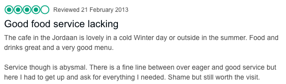
Figure 4-2. A review that praises some aspects and criticizes few
Would you call the review in Figure 4-2 negative, positive, or neutral? It’s difficult to answer this—the food was great, but the service was bad. Practitioners and brands working with sentiment analysis have realized that many products or services have multiple facets. In order to understand overall sentiment, understanding each and every facet is important. Text classification plays a major role in performing such fine-grained analysis of customer feedback. We’ll discuss this specific application in detail in Chapter 9.
- Other applications
Apart from the above-mentioned areas, text classification is also used in several other applications in various domains:
-
Text classification is used in language identification, like identifying the language of new tweets or posts. For example, Google Translate has an automatic language identification feature.
-
Authorship attribution, or identifying the unknown authors of texts from a pool of authors, is another popular use case of text classification, and it’s used in a range of fields from forensic analysis to literary studies.
-
Text classification has been used in the recent past for triaging posts in an online support forum for mental health services [4]. In the NLP community, annual competitions are conducted (e.g., clpsych.org) for solving such text classification problems originating from clinical research.
-
In the recent past, text classification has also been used to segregate fake news from real news.
-
Note that this section only serves as an illustration of the wide range of applications of text classification, and the list is not exhaustive, but we hope it gives you enough background to identify text classification problems in your workplace projects when you encounter them. Let’s now look at how to build such text classification models.
A Pipeline for Building Text Classification Systems
In Chapter 2, we discussed some of the common NLP pipelines. The text classification pipeline shares some of its steps with the pipelines we learned in that chapter.
One typically follows these steps when building a text classification system:
-
Collect or create a labeled dataset suitable for the task.
-
Split the dataset into two (training and test) or three parts: training, validation (i.e., development), and test sets, then decide on evaluation metric(s).
-
Transform raw text into feature vectors.
-
Train a classifier using the feature vectors and the corresponding labels from the training set.
-
Using the evaluation metric(s) from Step 2, benchmark the model performance on the test set.
-
Deploy the model to serve the real-world use case and monitor its performance.
Figure 4-3 shows these typical steps in building a text classification system.
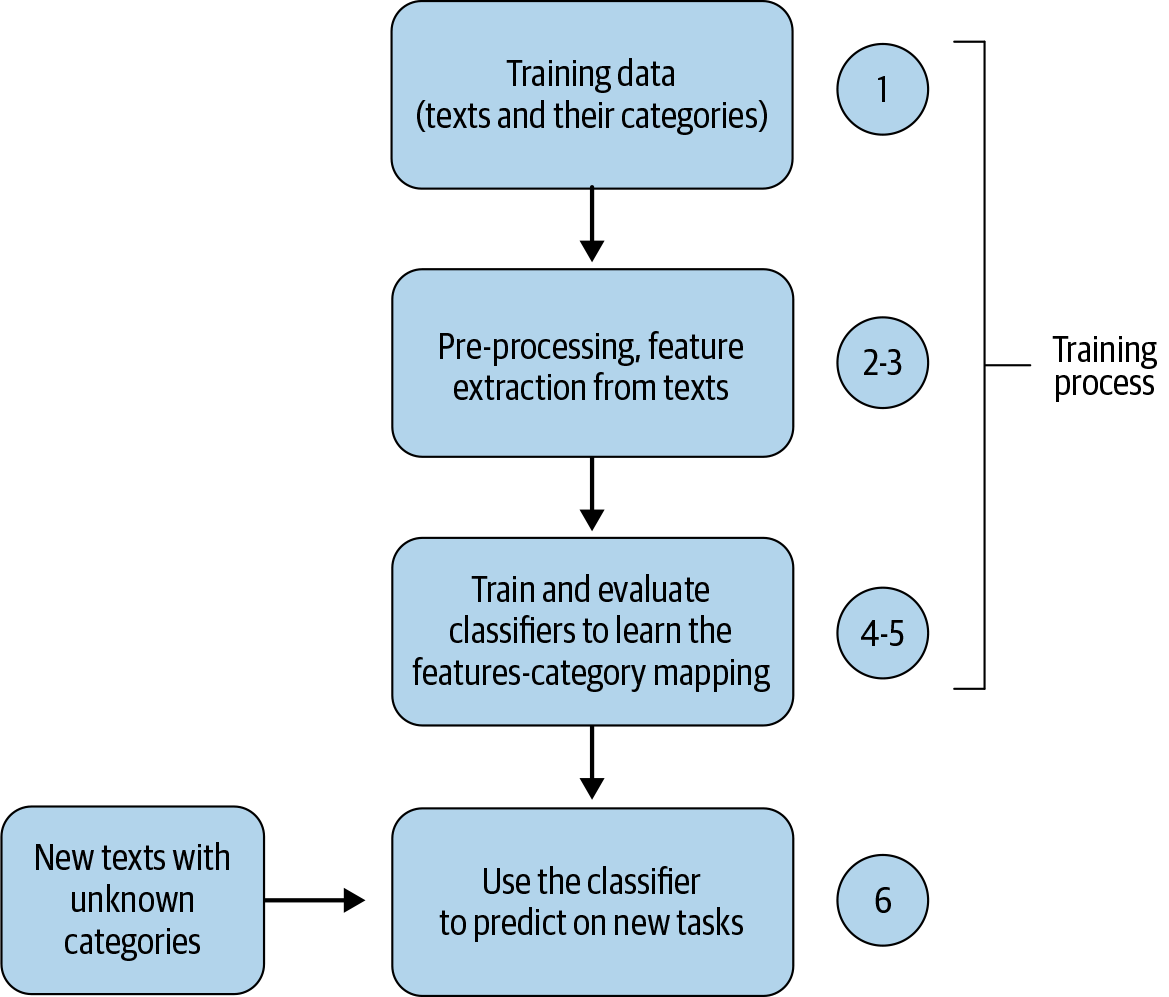
Figure 4-3. Flowchart of a text classification pipeline
Steps 3 through 5 are iterated on to explore different variants of features and classification algorithms and their parameters and to tune the hyperparameters before proceeding to Step 6, deploying the optimal model in production.
Some of the individual steps related to data collection and pre-processing were discussed in past chapters. For example, Steps 1 and 2 were discussed in detail in Chapter 2. Chapter 3 focused entirely on Step 3. Our focus in this chapter is on Steps 4 through 5. Toward the end of this chapter, we’ll revisit Step 1 to discuss issues specific to text classification. We’ll deal with Step 6 in Chapter 11. To be able to perform Steps 4 through 5 (i.e., to benchmark the performance of a model or compare multiple classifiers), we need the right measure(s) of evaluation. Chapter 2 discussed various general metrics used in evaluating NLP systems. For evaluating classifiers specifically, among the metrics introduced in Chapter 2, the following are used more commonly: classification accuracy, precision, recall, F1 score, and area under ROC curve. In this chapter, we’ll use some of these measures to evaluate our models and also look at confusion matrices to understand the model performance in detail.
Apart from these, when classification systems are deployed in real-world applications, key performance indicators (KPIs) specific to a given business use case are also used to evaluate their impact and return on investment (ROI). These are often the metrics business teams care about. For example, if we’re using text classification to automatically route customer service requests, a possible KPI could be the reduction in wait time before the request is responded to compared to manual routing. In this chapter, we’ll focus on the NLP evaluation measures. In Part III of the book, where we’ll discuss NLP use cases specific to industry verticals, we’ll introduce some KPIs that are often used in those verticals.
Before we start looking at how to build text classifiers using the pipeline we just discussed, let’s take a look at the scenarios where this pipeline is not at all necessary or where it’s not possible to use it.
A Simple Classifier Without the Text Classification Pipeline
When we talk about the text classification pipeline, we’re referring to a supervised machine learning scenario. However, it’s possible to build a simple classifier without machine learning and without this pipeline. Consider the following problem scenario: we’re given a corpus of tweets where each tweet is labeled with its corresponding sentiment: negative or positive. For example, a tweet that says, “The new James Bond movie is great!” is clearly expressing a positive sentiment, whereas a tweet that says, “I would never visit this restaurant again, horrible place!!” has a negative sentiment. We want to build a classification system that will predict the sentiment of an unseen tweet using only the text of the tweet. A simple solution could be to create lists of positive and negative words in English—i.e., words that have a positive or negative sentiment. We then compare the usage of positive versus negative words in the input tweet and make a prediction based on this information. Further enhancements to this approach may involve creating more sophisticated dictionaries with degrees of positive, negative, and neutral sentiment of words or formulating specific heuristics (e.g., usage of certain smileys indicate positive sentiment) and using them to make predictions. This approach is called lexicon-based sentiment analysis.
Clearly, this does not involve any “learning” of text classification; that is, it’s based on a set of heuristics or rules and custom-built resources such as dictionaries of words with sentiment. While this approach may seem too simple to perform reasonably well for many real-world scenarios, it may enable us to deploy a minimum viable product (MVP) quickly. Most importantly, this simple model can lead to better understanding of the problem and give us a simple baseline for our evaluation metric and speed. From our experience, it’s always good to start with such simpler approaches when tackling a new NLP problem, where possible. However, eventually, we’ll need ML methods that can infer more insights from large collections of text data and perform better than the baseline approach.
Using Existing Text Classification APIs
Another scenario where we may not have to “learn” a classifier or follow this pipeline is when our task is more generic in nature, such as identifying a general category of a text (e.g., whether it’s about technology or music). In such cases, we can use existing APIs, such as Google Cloud Natural Language [5], that provide off-the-shelf content classification models that can identify close to 700 different categories of text. Another popular classification task is sentiment analysis. All major service providers (e.g., Google, Microsoft, and Amazon) serve sentiment analysis APIs [5, 6, 7] with varying payment structures. If we’re tasked with building a sentiment classifier, we may not have to build our own system if an existing API addresses our business needs.
However, many classification tasks could be specific to our organization’s business needs. For the rest of this chapter, we’ll address the scenario of building our own classifier by considering the pipeline described earlier in this section.
One Pipeline, Many Classifiers
Let’s now look at building text classifiers by altering Steps 3 through 5 in the pipeline and keeping the remaining steps constant. A good dataset is a prerequisite to start using the pipeline. When we say “good” dataset, we mean a dataset that is a true representation of the data we’re likely to see in production. Throughout this chapter, we’ll use some of the publicly available datasets for text classification. A wide range of NLP-related datasets, including ones for text classification, are listed online [8]. Additionally, Figure Eight [9] contains a collection of crowdsourced datasets, some of which are relevant to text classification. The UCI Machine Learning Repository [10] also contains a few text classification datasets. Google recently launched a dedicated search system for datasets for machine learning [11]. We’ll use multiple datasets throughout this chapter instead of sticking to one to illustrate any dataset-specific issues you may come across.
Note that our goal in this chapter is to give you an overview of different approaches. No single approach is known to work universally well on all kinds of data and all classification problems. In the real world, we experiment with multiple approaches, evaluate them, and choose one final approach to deploy in practice.
For the rest of this section, we’ll use the “Economic News Article Tone and Relevance” dataset from Figure Eight to demonstrate text classification. It consists of 8,000 news articles annotated with whether or not they’re relevant to the US economy (i.e., a yes/no binary classification). The dataset is also imbalanced, with ~1,500 relevant and ~6,500 non-relevant articles, which poses the challenge of guarding against learning a bias toward the majority category (in this case, non-relevant articles). Clearly, learning what a relevant news article is is more challenging with this dataset than learning what is irrelevant. After all, just guessing that everything is irrelevant already gives us 80% accuracy!
Let’s explore how a BoW representation (introduced in Chapter 3) can be used with this dataset following the pipeline described earlier in this chapter. We’ll build classifiers using three well-known algorithms: Naive Bayes, logistic regression, and support vector machines. The notebook related to this section (Ch4/OnePipeline_ManyClassifiers.ipynb) shows the step-by-step process of following our pipeline using these three algorithms. We’ll discuss some of the important aspects in this section.
Naive Bayes Classifier
Naive Bayes is a probabilistic classifier that uses Bayes’ theorem to classify texts based on the evidence seen in training data. It estimates the conditional probability of each feature of a given text for each class based on the occurrence of that feature in that class and multiplies the probabilities of all the features of a given text to compute the final probability of classification for each class. Finally, it chooses the class with maximum probability. A detailed step-by-step explanation of the classifier is beyond the scope of this book. However, a reader interested in Naive Bayes with a detailed explanation in the context of text classification can look at Chapter 4 of Jurafsky and Martin [12]. Although simple, Naive Bayes is commonly used as a baseline algorithm in classification experiments.
Let’s walk through the key steps of an implementation of the pipeline described earlier for our dataset. For this, we use a Naive Bayes implementation in scikit-learn. Once the dataset is loaded, we split the data into train and test data, as shown in the code snippet below:
#Step 1: train-test splitX=our_data.text#the column text contains textual data to extract features from.y=our_data.relevance#this is the column we are learning to predict.X_train,X_test,y_train,y_test=train_test_split(X,y,random_state=1)#split X and y into training and testing sets. By default,itsplits75%#training and 25% test. random_state=1 for reproducibility.
The next step is to pre-process the texts and then convert them into feature vectors. While there are many different ways to do the pre-processing, let’s say we want to do the following: lowercasing and removal of punctuation, digits and any custom strings, and stop words. The code snippet below shows this pre-processing and converting the train and test data into feature vectors using CountVectorizer in scikit-learn, which is the implementation of the BoW approach we discussed in Chapter 3:
#Step 2-3: Pre-process and Vectorize train and test datavect=CountVectorizer(preprocessor=clean)#clean is a function we defined for pre-processing, seen in the notebook.X_train_dtm=vect.fit_transform(X_train)X_test_dtm=vect.transform(X_test)(X_train_dtm.shape,X_test_dtm.shape)
Once we run this in the notebook, we’ll see that we ended up having a feature vector with over 45,000 features! We now have the data in a format we want: feature vectors. So, the next step is to train and evaluate a classifier. The code snippet below shows how to do the training and evaluation of a Naive Bayes classifier with the features we extracted above:
nb=MultinomialNB()#instantiate a Multinomial Naive Bayes classifiernb.fit(X_train_dtm,y_train)#train the modey_pred_class=nb.predict(X_test_dtm)#make class predictions for test data
Figure 4-4 shows the confusion matrix of this classifier with test data.
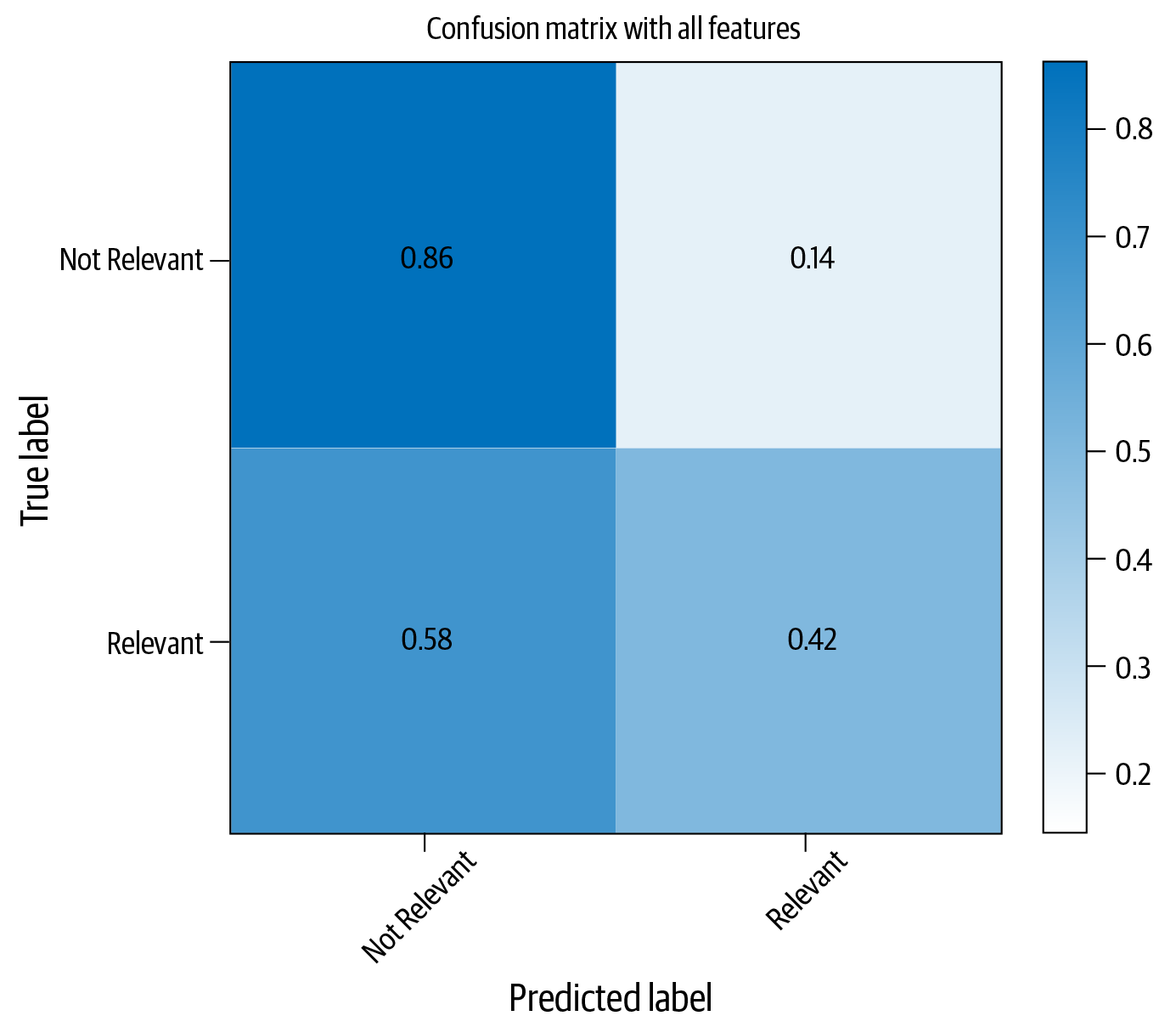
Figure 4-4. Confusion matrix for Naive Bayes classifier
As evident from Figure 4-4, the classifier is doing fairly well with identifying the non-relevant articles correctly, only making errors 14% of the time. However, it does not perform well in comparison to the second category: relevance. The category is identified correctly only 42% of the time. An obvious thought may be to collect more data. This is correct and often the most rewarding approach. But in the interest of covering other approaches, we assume that we cannot change it or collect additional data. This is not a far-fetched assumption—in industry, we often don’t have the luxury of collecting more data; we have to work with what we have. We can think of a few possible reasons for this performance and ways to improve this classifier. These are summarized in Table 4-1, and we’ll look into some of them as we progress in this chapter.
| Reason 1 | Since we extracted all possible features, we ended up in a large, sparse feature vector, where most features are too rare and end up being noise. A sparse feature set also makes training hard. |
| Reason 2 | There are very few examples of relevant articles (~20%) compared to the non-relevant articles (~80%) in the dataset. This class imbalance makes the learning process skewed toward the non-relevant articles category, as there are very few examples of “relevant” articles. |
| Reason 3 | Perhaps we need a better learning algorithm. |
| Reason 4 | Perhaps we need a better pre-processing and feature extraction mechanism. |
| Reason 5 | Perhaps we should look to tuning the classifier’s parameters and hyperparameters. |
Let’s see how to improve our classification performance by addressing some of the possible reasons for it. One way to approach Reason 1 is to reduce noise in the feature vectors. The approach in the previous code example had close to 40,000 features (refer to the Jupyter notebook for details). A large number of features introduce sparsity; i.e., most of the features in the feature vector are zero, and only a few values are non-zero. This, in turn, affects the ability of the text classification algorithm to learn. Let’s see what happens if we restrict this to 5,000 and rerun the training and evaluation process. This requires us to change the CountVectorizer instantiation in the process, as shown in the code snippet below, and repeat all the steps:
vect=CountVectorizer(preprocessor=clean,max_features=5000)#Step-1X_train_dtm=vect.fit_transform(X_train)#combined step 2 and 3X_test_dtm=vect.transform(X_test)nb=MultinomialNB()#instantiate a Multinomial Naive Bayes model%timenb.fit(X_train_dtm,y_train)#train the model(timing it with an IPython "magic command")y_pred_class=nb.predict(X_test_dtm)#make class predictions for X_test_dtm("Accuracy: ",metrics.accuracy_score(y_test,y_pred_class))
Figure 4-5 shows the new confusion matrix with this setting.
Now, clearly, while the average performance seems lower than before, the correct identification of relevant articles increased by over 20%. At that point, one may wonder whether this is what we want. The answer to that question depends on the problem we’re trying to solve. If we care about doing reasonably well with non-relevant article identification and doing as well as possible with relevant article identification, or doing equally well with both, we could conclude that reducing the feature vector size with the Naive Bayes classifier was useful for this dataset.
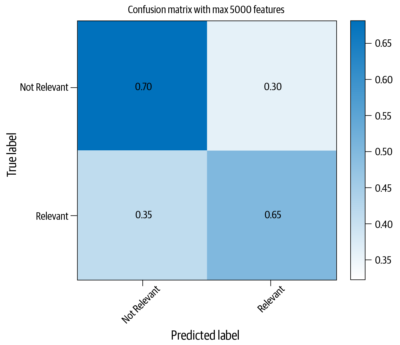
Figure 4-5. Improved classification performance with Naive Bayes and feature selection
Tip
Consider reducing the number of features if there are too many to reduce data sparsity.
Reason 2 in our list was the problem of skew in data toward the majority class. There are several ways to address this. Two typical approaches are oversampling the instances belonging to minority classes or undersampling the majority class to create a balanced dataset. Imbalanced-Learn [13] is a Python library that incorporates some of the sampling methods to address this issue. While we won’t delve into the details of this library here, classifiers also have a built-in mechanism to address such imbalanced datasets. We’ll see how to use that by taking another classifier, logistic regression, in the next subsection.
Tip
Class imbalance is one of the most common reasons for a classifier to not do well. We must always check if this is the case for our task and address it.
To address Reason 3, let’s try using other algorithms, beginning with logistic regression.
Logistic Regression
When we described the Naive Bayes classifier, we mentioned that it learns the probability of a text for each class and chooses the one with maximum probability. Such a classifier is called a generative classifier. In contrast, there’s a discriminative classifier that aims to learn the probability distribution over all classes. Logistic regression is an example of a discriminative classifier and is commonly used in text classification, as a baseline in research, and as an MVP in real-world industry scenarios.
Unlike Naive Bayes, which estimates probabilities based on feature occurrence in classes, logistic regression “learns” the weights for individual features based on how important they are to make a classification decision. The goal of logistic regression is to learn a linear separator between classes in the training data with the aim of maximizing the probability of the data. This “learning” of feature weights and probability distribution over all classes is done through a function called “logistic” function, and (hence the name) logistic regression [14].
Let’s take the 5,000-dimensional feature vector from the last step of the Naive Bayes example and train a logistic regression classifier instead of Naive Bayes. The code snippet below shows how to use logistic regression for this task:
fromsklearn.linear_modelimportLogisticRegressionlogreg=LogisticRegression(class_weight="balanced")logreg.fit(X_train_dtm,y_train)y_pred_class=logreg.predict(X_test_dtm)("Accuracy: ",metrics.accuracy_score(y_test,y_pred_class))
This results in a classifier with an accuracy of 73.7%. Figure 4-6 shows the confusion matrix with this approach.
Our logistic regression classifier instantiation has an argument class_weight, which is given a value “balanced”. This tells the classifier to boost the weights for classes in inverse proportion to the number of samples for that class. So, we expect to see better performance for the less-represented classes. We can experiment with this code by removing that argument and retraining the classifier, to witness a fall (by approximately 5%) in the bottom-right cell of the confusion matrix. However, logistic regression clearly seems to perform worse than Naive Bayes for this dataset.
Reason 3 in our list was: “Perhaps we need a better learning algorithm.” This gives rise to the question: “What is a better learning algorithm?” A general rule of thumb when working with ML approaches is that there is no one algorithm that learns well on all datasets. A common approach is to experiment with various algorithms and compare them.
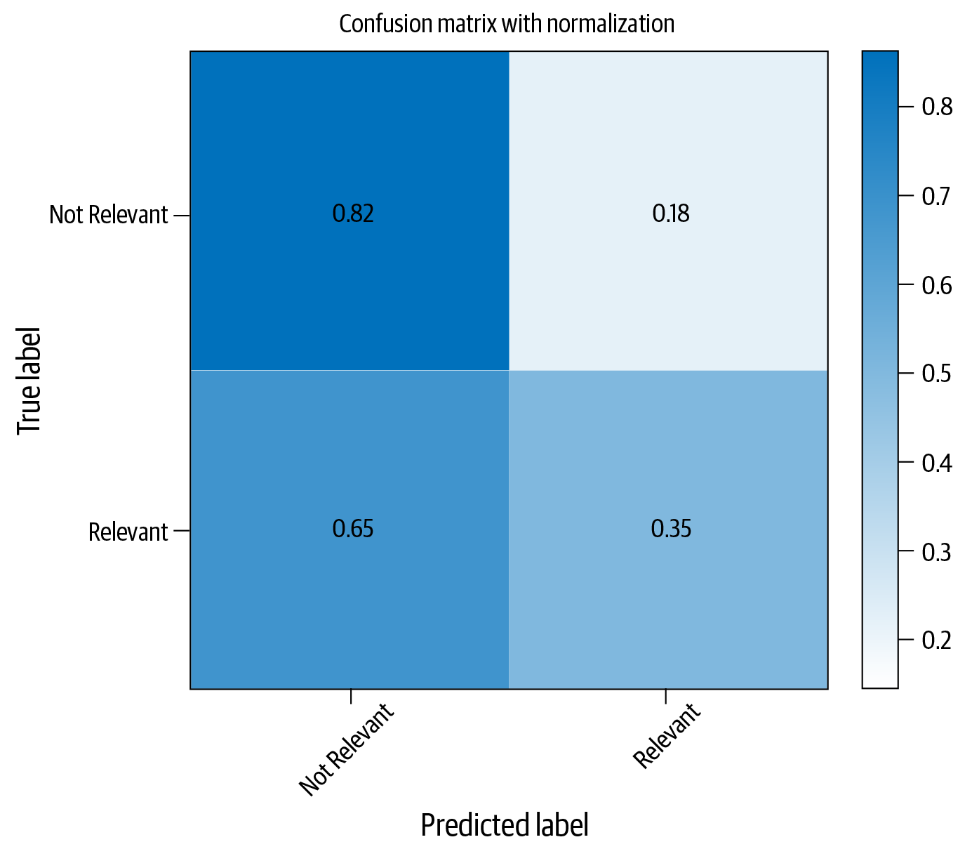
Figure 4-6. Classification performance with logistic regression
Let’s see if this idea helps us by replacing logistic regression with another well-known classification algorithm that was shown to be useful for several text classification tasks, called the “support vector machine.”
Support Vector Machine
We described logistic regression as a discriminative classifier that learns the weights for individual features and predicts a probability distribution over the classes. A support vector machine (SVM), first invented in the early 1960s, is a discriminative classifier like logistic regression. However, unlike logistic regression, it aims to look for an optimal hyperplane in a higher dimensional space, which can separate the classes in the data by a maximum possible margin. Further, SVMs are capable of learning even non-linear separations between classes, unlike logistic regression. However, they may also take longer to train.
SVMs come in various flavors in sklearn. Let’s see how one of them is used by keeping everything else the same and altering maximum features to 1,000 instead of the previous example’s 5,000. We restrict to 1,000 features, keeping in mind the time an SVM algorithm takes to train. The code snippet below shows how to do this, and Figure 4-7 shows the resultant confusion matrix:
fromsklearn.svmimportLinearSVCvect=CountVectorizer(preprocessor=clean,max_features=1000)#Step-1X_train_dtm=vect.fit_transform(X_train)#combined step 2 and 3X_test_dtm=vect.transform(X_test)classifier=LinearSVC(class_weight='balanced')#notice the “balanced” optionclassifier.fit(X_train_dtm,y_train)#fit the model with training datay_pred_class=classifier.predict(X_test_dtm)("Accuracy: ",metrics.accuracy_score(y_test,y_pred_class))

Figure 4-7. Confusion matrix for classification with SVM
When compared to logistic regression, SVMs seem to have done better with the relevant articles category, although, among this small set of experiments we did, Naive Bayes, with the smaller set of features, seems to be the best classifier for this dataset.
All the examples in this section demonstrate how changes in different steps affected the classification performance and how to interpret the results. Clearly, we excluded many other possibilities, such as exploring other text classification algorithms, changing different parameters of various classifiers, coming up with better pre-processing methods, etc. We leave them as further exercises for the reader, using the notebook as a playground. A real-world text classification project involves exploring multiple options like this, starting with the simplest approach in terms of modeling, deployment, and scaling, and gradually increasing the complexity. Our eventual goal is to build the classifier that best meets our business needs given all the other constraints.
Let’s now consider a part of Reason 4 in Table 4-1: better feature representation. So far in this chapter, we’ve used BoW features. Let’s see how we can use other feature representation techniques we saw in Chapter 3 for text classification.
Using Neural Embeddings in Text Classification
In the latter half of Chapter 3, we discussed feature engineering techniques using neural networks, such as word embeddings, character embeddings, and document embeddings. The advantage of using embedding-based features is that they create a dense, low-dimensional feature representation instead of the sparse, high-dimensional structure of BoW/TF-IDF and other such features. There are different ways of designing and using features based on neural embeddings. In this section, let’s look at some ways of using such embedding representations for text classification.
Word Embeddings
Words and n-grams have been used primarily as features in text classification for a long time. Different ways of vectorizing words have been proposed, and we used one such representation in the last section, CountVectorizer. In the past few years, neural network–based architectures have become popular for “learning” word representations, which are known as “word embeddings.” We surveyed some of the intuitions behind this in Chapter 3. Let’s now take a look at how to use word embeddings as features for text classification. We’ll use the sentiment-labeled sentences dataset from the UCI repository, consisting of 1,500 positive-sentiment and 1,500 negative-sentiment sentences from Amazon, Yelp, and IMDB. All the steps are detailed in the notebook Ch4/Word2Vec_Example.ipynb. Let’s walk through the important steps and where this approach differs from the previous section’s procedures.
Loading and pre-processing the text data remains a common step. However, instead of vectorizing the texts using BoW-based features, we’ll now rely on neural embedding models. As mentioned earlier, we’ll use a pre-trained embedding model. Word2vec is a popular algorithm we discussed in Chapter 3 for training word embedding models. There are several pre-trained Word2vec models trained on large corpora available on the internet. Here, we’ll use the one from Google [15]. The following code snippet shows how to load this model into Python using gensim:
data_path="/your/folder/path"path_to_model=os.path.join(data_path,'GoogleNews-vectors-negative300.bin')training_data_path=os.path.join(data_path,"sentiment_sentences.txt")#Load W2V model. This will take some time.w2v_model=KeyedVectors.load_word2vec_format(path_to_model,binary=True)('done loading Word2Vec')
This is a large model that can be seen as a dictionary where the keys are words in the vocabulary and the values are their learned embedding representations. Given a query word, if the word’s embedding is present in the dictionary, it will return the same. How do we use this pre-learned embedding to represent features? As we discussed in Chapter 3, there are multiple ways of doing this. A simple approach is just to average the embeddings for individual words in text. The code snippet below shows a simple function to do this:
# Creating a feature vector by averaging all embeddings for all sentencesdefembedding_feats(list_of_lists):DIMENSION=300zero_vector=np.zeros(DIMENSION)feats=[]fortokensinlist_of_lists:feat_for_this=np.zeros(DIMENSION)count_for_this=0fortokenintokens:iftokeninw2v_model:feat_for_this+=w2v_model[token]count_for_this+=1feats.append(feat_for_this/count_for_this)returnfeatstrain_vectors=embedding_feats(texts_processed)(len(train_vectors))
Note that it uses embeddings only for the words that are present in the dictionary. It ignores the words for which embeddings are absent. Also, note that the above code will give a single vector with DIMENSION(=300) components. We treat the resulting embedding vector as the feature vector that represents the entire text. Once this feature engineering is done, the final step is similar to what we did in the previous section: use these features and train a classifier. We leave that as an exercise to the reader (refer to the notebook for the full code).
When trained with a logistic regression classifier, these features gave a classification accuracy of 81% on our dataset (see the notebook for more details). Considering that we just used an existing word embeddings model and followed only basic pre-processing steps, this is a great model to have as a baseline! We saw in Chapter 3 that there are other pre-trained embedding approaches, such as GloVe, which can be experimented with for this approach. Gensim, which we used in this example, also supports training our own word embeddings if necessary. If we’re working on a custom domain whose vocabulary is remarkably different from that of the pre-trained news embeddings we used here, it would make sense to train our own embeddings to extract features.
In order to decide whether to train our own embeddings or use pre-trained embeddings, a good rule of thumb is to compute the vocabulary overlap. If the overlap between the vocabulary of our custom domain and that of pre-trained word embeddings is greater than 80%, pre-trained word embeddings tend to give good results in text classification.
An important factor to consider when deploying models with embedding-based feature extraction approaches is that the learned or pre-trained embedding models have to be stored and loaded into memory while using these approaches. If the model itself is bulky (e.g., the pre-trained model we used takes 3.6 GB), we need to factor this into our deployment needs.
Subword Embeddings and fastText
Word embeddings, as the name indicates, are about word representations. Even off-the-shelf embeddings seem to work well on classification tasks, as we saw earlier. However, if a word in our dataset was not present in the pre-trained model’s vocabulary, how will we get a representation for this word? This problem is popularly known as out of vocabulary (OOV). In our previous example, we just ignored such words from feature extraction. Is there a better way?
We discussed fastText embeddings [16] in Chapter 3. They’re based on the idea of enriching word embeddings with subword-level information. Thus, the embedding representation for each word is represented as a sum of the representations of individual character n-grams. While this may seem like a longer process compared to just estimating word-level embeddings, it has two advantages:
-
This approach can handle words that did not appear in training data (OOV).
-
The implementation facilitates extremely fast learning on even very large corpora.
While fastText is a general-purpose library to learn the embeddings, it also supports off-the-shelf text classification by providing end-to-end classifier training and testing; i.e., we don’t have to handle feature extraction separately. The remaining part of this subsection shows how to use the fastText classifier [17] for text classification. We’ll work with the DBpedia dataset [18]. It’s a balanced dataset consisting of 14 classes, with 40,000 training and 5,000 testing examples per class. Thus, the total size of the dataset is 560,000 training and 70,000 testing data points. Clearly, this is a much larger dataset than what we saw before. Can we build a fast training model using fastText? Let’s check it out!
The training and test sets are provided as CSV files in this dataset. So, the first step involves reading these files into your Python environment and cleaning the text to remove extraneous characters, similar to what we did in the pre-processing steps for the other classifier examples we’ve seen so far. Once this is done, the process to use fastText is quite simple. The code snippet below shows a simple fastText model. The step-by-step process is detailed in the associated Jupyter notebook (Ch4/FastText_Example.ipynb):
## Using fastText for feature extraction and trainingfromfasttextimportsupervised"""fastText expects and training file (csv), a model name as input arguments.label_prefix refers to the prefix before label string in the dataset.default is __label__. In our dataset, it is __class__.There are several other parameters which can be seen in:https://pypi.org/project/fasttext/"""model=supervised(train_file,'temp',label_prefix="__class__")results=model.test(test_file)(results.nexamples,results.precision,results.recall)
If we run this code in the notebook, we’ll notice that, despite the fact that this is a huge dataset and we gave the classifier raw text and not the feature vector, the training takes only a few seconds, and we get close to 98% precision and recall! As an exercise, try to build a classifier using the same dataset but with either BoW or word embedding features and algorithms like logistic regression. Notice how long it takes for the individual steps of feature extraction and classification learning!
When we have a large dataset, and when learning seems infeasible with the approaches described so far, fastText is a good option to use to set up a strong working baseline. However, there’s one concern to keep in mind when using fastText, as was the case with Word2vec embeddings: it uses pre-trained character n-gram embeddings. Thus, when we save the trained model, it carries the entire character n-gram embeddings dictionary with it. This results in a bulky model and can result in engineering issues. For example, the model stored with the name “temp” in the above code snippet has a size close to 450 MB. However, fastText implementation also comes with options to reduce the memory footprint of its classification models with minimal reduction in classification performance [19]. It does this by doing vocabulary pruning and using compression algorithms. Exploring these possibilities could be a good option in cases where large model sizes are a constraint.
Tip
fastText is extremely fast to train and very useful for setting up strong baselines. The downside is the model size.
We hope this discussion gives a good overview of the usefulness of fastText for text classification. What we showed here is a default classification model without any tuning of the hyperparameters. fastText’s documentation contains more information on the different options to tune your classifier and on training custom embedding representations for a dataset you want. However, both of the embedding representations we’ve seen so far learn a representation of words and characters and collect them together to form a text representation. Let’s see how to learn the representation for a document directly using the Doc2vec approach we discussed in Chapter 3.
Document Embeddings
In the Doc2vec embedding scheme, we learn a direct representation for the entire document (sentence/paragraph) rather than each word. Just as we used word and character embeddings as features for performing text classification, we can also use Doc2vec as a feature representation mechanism. Since there are no existing pre-trained models that work with the latest version of Doc2vec [20], let’s see how to build our own Doc2vec model and use it for text classification.
We’ll use a dataset called “Sentiment Analysis: Emotion in Text” from figure-eight.com [9], which contains 40,000 tweets labeled with 13 labels signifying different emotions. Let’s take the three most frequent labels in this dataset—neutral, worry, happiness—and build a text classifier for classifying new tweets into one of these three classes. The notebook for this subsection (Ch4/Doc2Vec_Example.ipynb) walks you through the steps involved in using Doc2vec for text classification and provides the dataset.
After loading the dataset and taking a subset of the three most frequent labels, an important step to consider here is pre-processing the data. What’s different here compared to previous examples? Why can’t we just follow the same procedure as before? There are a few things that are different about tweets compared to news articles or other such text, as we briefly discussed in Chapter 2 when we talked about text pre-processing. First, they are very short. Second, our traditional tokenizers may not work well with tweets, splitting smileys, hashtags, Twitter handles, etc., into multiple tokens. Such specialized needs prompted a lot of research into NLP for Twitter in the recent past, which resulted in several pre-processing options for tweets. One such solution is a TweetTokenizer, implemented in the NLTK [21] library in Python. We’ll discuss more on this topic in Chapter 8. For now, let’s see how we can use a TweetTokenizer in the following code snippet:
tweeter=TweetTokenizer(strip_handles=True,preserve_case=False)mystopwords=set(stopwords.words("english"))#Function to pre-process and tokenize tweetsdefpreprocess_corpus(texts):defremove_stops_digits(tokens):#Nested function to remove stopwords and digitsreturn[tokenfortokenintokensiftokennotinmystopwordsandnottoken.isdigit()]return[remove_stops_digits(tweeter.tokenize(content))forcontentintexts]mydata=preprocess_corpus(df_subset['content'])mycats=df_subset['sentiment']
The next step in this process is to train a Doc2vec model to learn tweet representations. Ideally, any large dataset of tweets will work for this step. However, since we don’t have such a ready-made corpus, we’ll split our dataset into train-test and use the training data for learning the Doc2vec representations. The first part of this process involves converting the data into a format readable by the Doc2vec implementation, which can be done using the TaggedDocument class. It’s used to represent a document as a list of tokens, followed by a “tag,” which in its simplest form can be just the filename or ID of the document. However, Doc2vec by itself can also be used as a nearest neighbor classifier for both multiclass and multilabel classification problems using . We’ll leave this as an exploratory exercise for the reader. Let’s now see how to train a Doc2vec classifier for tweets through the code snippet below:
#Prepare training data in doc2vec format:d2vtrain=[TaggedDocument((d),tags=[str(i)])fori,dinenumerate(train_data)]#Train a doc2vec model to learn tweet representations. Use only training data!!model=Doc2Vec(vector_size=50,alpha=0.025,min_count=10,dm=1,epochs=100)model.build_vocab(d2vtrain)model.train(d2vtrain,total_examples=model.corpus_count,epochs=model.epochs)model.save("d2v.model")("Model Saved")
Training for Doc2vec involves making several choices regarding parameters, as seen in the model definition in the code snippet above. vector_size refers to the dimensionality of the learned embeddings; alpha is the learning rate; min_count is the minimum frequency of words that remain in vocabulary; dm, which stands for distributed memory, is one of the representation learners implemented in Doc2vec (the other is dbow, or distributed bag of words); and epochs are the number of training iterations. There are a few other parameters that can be customized. While there are some guidelines on choosing optimal parameters for training Doc2vec models [22], these are not exhaustively validated, and we don’t know if the guidelines work for tweets.
The best way to address this issue is to explore a range of values for the ones that matter to us (e.g., dm versus dbow, vector sizes, learning rate) and compare multiple models. How do we compare these models, as they only learn the text representation? One way to do it is to start using these learned representations in a downstream task—in this case, text classification. Doc2vec’s infer_vector function can be used to infer the vector representation for a given text using a pre-trained model. Since there is some amount of randomness due to the choice of hyperparameters, the inferred vectors differ each time we extract them. For this reason, to get a stable representation, we run it multiple times (called steps) and aggregate the vectors. Let’s use the learned model to infer features for our data and train a logistic regression classifier:
#Infer the feature representation for training and test data using#the trained modelmodel=Doc2Vec.load("d2v.model")#Infer in multiple steps to get a stable representationtrain_vectors=[model.infer_vector(list_of_tokens,steps=50)forlist_of_tokensintrain_data]test_vectors=[model.infer_vector(list_of_tokens,steps=50)forlist_of_tokensintest_data]myclass=LogisticRegression(class_weight="balanced")#because classes are not balancedmyclass.fit(train_vectors,train_cats)preds=myclass.predict(test_vectors)(classification_report(test_cats,preds))
Now, the performance of this model seems rather poor, achieving an F1 score of 0.51 on a reasonably large corpus, with only three classes. There are a couple of interpretations for this poor result. First, unlike full news articles or even well-formed sentences, tweets contain very little data per instance. Further, people write with a wide variety in spelling and syntax when they tweet. There are a lot of emoticons in different forms. Our feature representation should be able to capture such aspects. While tuning the algorithms by searching a large parameter space for the best model may help, an alternative could be to explore problem-specific feature representations, as we discussed in Chapter 3. We’ll see how to do this for tweets in Chapter 8. An important point to keep in mind when using Doc2vec is the same as for fastText: if we have to use Doc2vec for feature representation, we have to store the model that learned the representation. While it’s not typically as bulky as fastText, it’s also not as fast to train. Such trade-offs need to be considered and compared before we make a deployment decision.
So far, we’ve seen a range of feature representations and how they play a role for text classification using ML algorithms. Let’s now turn to a family of algorithms that became popular in the past few years, known as “deep learning.”
Deep Learning for Text Classification
As we discussed in Chapter 1, deep learning is a family of machine learning algorithms where the learning happens through different kinds of multilayered neural network architectures. Over the past few years, it has shown remarkable improvements on standard machine learning tasks, such as image classification, speech recognition, and machine translation. This has resulted in widespread interest in using deep learning for various tasks, including text classification. So far, we’ve seen how to train different machine learning classifiers, using BoW and different kinds of embedding representations. Now, let’s look at how to use deep learning architectures for text classification.
Two of the most commonly used neural network architectures for text classification are convolutional neural networks (CNNs) and recurrent neural networks (RNNs). Long short-term memory (LSTM) networks are a popular form of RNNs. Recent approaches also involve starting with large, pre-trained language models and fine-tuning them for the task at hand. In this section, we’ll learn how to train CNNs and LSTMs and how to tune a pre-trained language model for text classification using the IMDB sentiment classification dataset [23]. Note that a detailed discussion on how neural network architectures work is beyond the scope of this book. Interested readers can read the textbook by Goodfellow et al. [24] for a general theoretical discussion and Goldberg’s book [25] for NLP-specific uses of neural network architectures. Jurafsky and Martin’s book [12] also provides a short but concise overview of different neural network methods for NLP.
The first step toward training any ML or DL model is to define a feature representation. This step has been relatively straightforward in the approaches we’ve seen so far, with BoW or embedding vectors. However, for neural networks, we need further processing of input vectors, as we saw in Chapter 3. Let’s quickly recap the steps involved in converting training and test data into a format suitable for the neural network input layers:
-
Tokenize the texts and convert them into word index vectors.
-
Pad the text sequences so that all text vectors are of the same length.
-
Map every word index to an embedding vector. We do that by multiplying word index vectors with the embedding matrix. The embedding matrix can either be populated using pre-trained embeddings or it can be trained for embeddings on this corpus.
-
Use the output from Step 3 as the input to a neural network architecture.
Once these are done, we can proceed with the specification of neural network architectures and training classifiers with them. The Jupyter notebook associated with this section (Ch4/DeepNN_Example.ipynb) will walk you through the entire process from text pre-processing to neural network training and evaluation. We’ll use Keras, a Python-based DL library. The code snippet below illustrates Steps 1 and 2:
#Vectorize these text samples into a 2D integer tensor using Keras Tokenizer.#Tokenizer is fit on training data only, and that is used to tokenize both train#and test data.tokenizer=Tokenizer(num_words=MAX_NUM_WORDS)tokenizer.fit_on_texts(train_texts)train_sequences=tokenizer.texts_to_sequences(train_texts)test_sequences=tokenizer.texts_to_sequences(test_texts)word_index=tokenizer.word_index('Found%sunique tokens.'%len(word_index))#Converting this to sequences to be fed into neural network. Max seq. len is#1000 as set earlier. Initial padding of 0s, until vector is of#size MAX_SEQUENCE_LENGTHtrainvalid_data=pad_sequences(train_sequences,maxlen=MAX_SEQUENCE_LENGTH)test_data=pad_sequences(test_sequences,maxlen=MAX_SEQUENCE_LENGTH)trainvalid_labels=to_categorical(np.asarray(train_labels))test_labels=to_categorical(np.asarray(test_labels))
Step 3: If we want to use pre-trained embeddings to convert the train and test data into an embedding matrix like we did in the earlier examples with Word2vec and fastText, we have to download them and use them to convert our data into the input format for the neural networks. The following code snippet shows an example of how to do this using GloVe embeddings, which were introduced in Chapter 3. GloVe embeddings come with multiple dimensionalities, and we chose 100 as our dimension here. The value of dimensionality is a hyperparameter, and we can experiment with other dimensions as well:i
embeddings_index={}withopen(os.path.join(GLOVE_DIR,'glove.6B.100d.txt'))asf:forlineinf:values=line.split()word=values[0]coefs=np.asarray(values[1:],dtype='float32')embeddings_index[word]=coefsnum_words=min(MAX_NUM_WORDS,len(word_index))+1embedding_matrix=np.zeros((num_words,EMBEDDING_DIM))forword,iinword_index.items():ifi>MAX_NUM_WORDS:continueembedding_vector=embeddings_index.get(word)ifembedding_vectorisnotNone:embedding_matrix[i]=embedding_vector
Step 4: Now, we’re ready to train DL models for text classification! DL architectures consist of an input layer, an output layer, and several hidden layers in between the two. Depending on the architecture, different hidden layers are used. The input layer for textual input is typically an embedding layer. The output layer, especially in the context of text classification, is a softmax layer with categorical output. If we want to train the input layer instead of using pre-trained embeddings, the easiest way is to call the Embedding layer class in Keras, specifying the input and output dimensions. However, since we want to use pre-trained embeddings, we should create a custom embedding layer that uses the embedding matrix we just built. The following code snippet shows how to do that:
embedding_layer=Embedding(num_words,EMBEDDING_DIM,embeddings_initializer=Constant(embedding_matrix),input_length=MAX_SEQUENCE_LENGTH,trainable=False)("Preparing of embedding matrix is done")
This will serve as the input layer for any neural network we want to use (CNN or LSTM). Now that we know how to pre-process the input and define an input layer, let’s move on to specifying the rest of the neural network architecture using CNNs and LSTMs.
CNNs for Text Classification
Let’s now look at how to define, train, and evaluate a CNN model for text classification. CNNs typically consist of a series of convolution and pooling layers as the hidden layers. In the context of text classification, CNNs can be thought of as learning the most useful bag-of-words/n-grams features instead of taking the entire collection of words/n-grams as features, as we did earlier in this chapter. Since our dataset has only two classes—positive and negative—the output layer has two outputs, with the softmax activation function. We’ll define a CNN with three convolution-pooling layers using the Sequential model class in Keras, which allows us to specify DL models as a sequential stack of layers—one after another. Once the layers and their activation functions are specified, the next task is to define other important parameters, such as the optimizer, loss function, and the evaluation metric to tune the hyperparameters of the model. Once all this is done, the next step is to train and evaluate the model. The following code snippet shows one way of specifying a CNN architecture for this task using the Python library Keras and prints the results with the IMDB dataset for this model:
('Define a 1D CNN model.')cnnmodel=Sequential()cnnmodel.add(embedding_layer)cnnmodel.add(Conv1D(128,5,activation='relu'))cnnmodel.add(MaxPooling1D(5))cnnmodel.add(Conv1D(128,5,activation='relu'))cnnmodel.add(MaxPooling1D(5))cnnmodel.add(Conv1D(128,5,activation='relu'))cnnmodel.add(GlobalMaxPooling1D())cnnmodel.add(Dense(128,activation='relu'))cnnmodel.add(Dense(len(labels_index),activation='softmax'))cnnmodel.compile(loss='categorical_crossentropy',optimizer='rmsprop',metrics=['acc'])cnnmodel.fit(x_train,y_train,batch_size=128,epochs=1,validation_data=(x_val,y_val))score,acc=cnnmodel.evaluate(test_data,test_labels)('Test accuracy with CNN:',acc)
As you can see, we made a lot of choices in specifying the model, such as activation functions, hidden layers, layer sizes, loss function, optimizer, metrics, epochs, and batch size. While there are some commonly recommended options for these, there’s no consensus on one combination that works best for all datasets and problems. A good approach while building your models is to experiment with different settings (i.e., hyperparameters). Keep in mind that all these decisions come with some associated cost. For example, in practice, we have the number of epochs as 10 or above. But that also increases the amount of time it takes to train the model. Another thing to note is that, if you want to train an embedding layer instead of using pre-trained embeddings in this model, the only thing that changes is the line cnnmodel.add(embedding_layer). Instead, we can specify a new embedding layer as, for example, cnnmodel.add(Embedding(Param1, Param2)). The code snippet below shows the code and model performance for the same:
("Defining and training a CNN model, training embedding layer on the flyinsteadofusingpre-trainedembeddings")cnnmodel=Sequential()cnnmodel.add(Embedding(MAX_NUM_WORDS,128))…...cnnmodel.fit(x_train,y_train,batch_size=128,epochs=1,validation_data=(x_val,y_val))score,acc=cnnmodel.evaluate(test_data,test_labels)('Test accuracy with CNN:',acc)
If we run this code in the notebook, we’ll notice that, in this case, training the embedding layer on our own dataset seems to result in better classification on test data. However, if the training data were substantially small, sticking to the pre-trained embeddings, or using the domain adaptation techniques we’ll discuss later in this chapter, would be a better choice. Let’s look at how to train similar models using an LSTM.
LSTMs for Text Classification
As we saw briefly in Chapter 1, LSTMs and other variants of RNNs in general have become the go-to way of doing neural language modeling in the past few years. This is primarily because language is sequential in nature and RNNs are specialized in working with sequential data. The current word in the sentence depends on its context—the words before and after. However, when we model text using CNNs, this crucial fact is not taken into account. RNNs work on the principle of using this context while learning the language representation or a model of language. Hence, they’re known to work well for NLP tasks. There are also CNN variants that can take such context into account, and CNNs versus RNNs is still an open area of debate. In this section, we’ll see an example of using RNNs for text classification. Now that we’ve already seen one neural network in action, it’s relatively easy to train another! Just replace the convolutional and pooling parts with an LSTM in the prior two code examples. The following code snippet shows how to train an LSTM model using the same IMDB dataset for text classification:
("Defining and training an LSTM model, training embedding layer on the fly")rnnmodel=Sequential()rnnmodel.add(Embedding(MAX_NUM_WORDS,128))rnnmodel.add(LSTM(128,dropout=0.2,recurrent_dropout=0.2))rnnmodel.add(Dense(2,activation='sigmoid'))rnnmodel.compile(loss='binary_crossentropy',optimizer='adam',metrics=['accuracy'])('Training the RNN')rnnmodel.fit(x_train,y_train,batch_size=32,epochs=1,validation_data=(x_val,y_val))score,acc=rnnmodel.evaluate(test_data,test_labels,batch_size=32)('Test accuracy with RNN:',acc)
Notice that this code took much longer to run than the CNN example. While LSTMs are more powerful in utilizing the sequential nature of text, they’re much more data hungry as compared to CNNs. Thus, the relative lower performance of the LSTM on a dataset need not necessarily be interpreted as a shortcoming of the model itself. It’s possible that the amount of data we have is not sufficient to utilize the full potential of an LSTM. As in the case of CNNs, several parameters and hyperparameters play important roles in model performance, and it’s always a good practice to explore multiple options and compare different models before finalizing on one.
Text Classification with Large, Pre-Trained Language Models
In the past two years, there have been great improvements in using neural network–based text representations for NLP tasks. We discussed some of these in “Universal Text Representations”. These representations have been used successfully for text classification in the recent past by fine-tuning the pre-trained models to the given task and dataset. BERT, which was mentioned in Chapter 3, is a popular model used in this way for text classification. Let’s take a look at how to use BERT for text classification using the IMDB dataset we used earlier in this section. The full code is in the relevant notebook (Ch4/BERT_Sentiment_Classification_IMDB.ipynb).
We’ll use ktrain, a lightweight wrapper to train and use pre-trained DL models using the TensorFlow library Keras. ktrain provides a straightforward process for all steps, from obtaining the dataset and the pre-trained BERT to fine-tuning it for the classification task. Let’s see how to load the dataset first through the code snippet below:
dataset=tf.keras.utils.get_file(fname="aclImdb.tar.gz",origin="http://ai.stanford.edu/~amaas/data/sentiment/aclImdb_v1.tar.gz",extract=True,)
Once the dataset is loaded, the next step is to download the BERT model and pre-process the dataset according to BERT’s requirements. The following code snippet shows how to do this with ktrain’s functions:
(x_train,y_train),(x_test,y_test),preproc=text.texts_from_folder(IMDB_DATADIR,maxlen=500,preprocess_mode='bert',train_test_names=['train','test'],
The next step is to load the pre-trained BERT model and fine-tune it for this dataset. Here’s the code snippet to do this:
model=text.text_classifier('bert',(x_train,y_train),preproc=preproc)learner=ktrain.get_learner(model,train_data=(x_train,y_train),val_data=(x_test,y_test),batch_size=6)learner.fit_onecycle(2e-5,4)
These three lines of code will train a text classifier using the BERT pre-trained model. As with other examples we’ve seen so far, we would need to do parameter tuning and a lot of experimentation to pick the best-performing model. We leave that as an exercise for the reader.
In this section, we introduced the idea of using DL for text classification using two neural network architectures—CNN and LSTM—and showed how we can tune a state-of-the-art, pre-trained language model (BERT) for a given dataset and classification task. There are several variants to these architectures, and new models are being proposed every day by NLP researchers. We saw how to use one pre-trained language model, BERT. There are other such models, and this is a constantly evolving area in NLP research; the state of the art keeps changing every few months (or even weeks!). However, in our experience as industry practitioners, several NLP tasks, especially text classification, still widely use several of the non-DL approaches we described earlier in the chapter. Two primary reasons for this are a lack of the large amounts of task-specific training data that neural networks demand and issues related to computing and deployment costs.
Tip
DL-based text classifiers are often nothing but condensed representations of the data they were trained on. These models are often as good as the training dataset. Selecting the right dataset becomes all the more important in such cases.
We’ll end this section by reiterating what we mentioned earlier when we discussed the text classification pipeline: in most industrial settings, it always makes sense to start with a simpler, easy-to-deploy approach as your MVP and go from there incrementally, taking customer needs and feasibility into account.
We’ve seen several approaches to building text classification models so far. Unlike heuristics-based approaches where the predictions can be justified by tracing back the rules applied on the data sample, ML models are treated as a black box while making predictions. However, in the recent past, the topic of interpretable ML started to gain prominence, and programs that can “explain” an ML model’s predictions exist now. Let’s take a quick look at their application for text classification.
Interpreting Text Classification Models
In the previous sections, we’ve seen how to train text classifiers using multiple approaches. In all these examples, we took the classifier predictions as is, without seeking any explanations. In fact, most real-world use cases of text classification may be similar—we just consume the classifier’s output and don’t question its decisions. Take spam classification: we generally don’t look for explanations of why a certain email is classified as spam or regular email. However, there may be scenarios where such explanations are necessary.
Consider a scenario where we developed a classifier that identifies abusive comments on a discussion forum website. The classifier identifies comments that are objectionable/abusive and performs the job of a human moderator by either deleting them or making them invisible to users. We know that classifiers aren’t perfect and can make errors. What if the commenter questions this moderation decision and asks for an explanation? Some method to “explain” the classification decision by pointing to which feature’s presence prompted such a decision can be useful in such cases. Such a method is also useful to provide some insights into the model and how it may perform on real-world data (instead of train/test sets), which may result in better, more reliable models in the future.
As ML models started getting deployed in real-world applications, interest in the direction of model interpretability grew. Recent research [26, 27] resulted in usable tools [28, 29] for interpreting model predictions (especially for classification). Lime [28] is one such tool that attempts to interpret a black-box classification model by approximating it with a linear model locally around a given training instance. The advantage of this is that such a linear model is expressed as a weighted sum of its features and is easy to interpret for humans. For example, if there are two features, f1 and f2, for a given test instance of a binary classifier with classes A and B, a Lime linear model around this instance could be something like -0.3 × f1 + 0.4 × f2 with a prediction B. This indicates that the presence of feature f1 will negatively affect this prediction (by 0.3) and skew it toward A. [26] explains this in more detail. Let’s now look at how Lime [28] can be used to understand the predictions of a text classifier.
Explaining Classifier Predictions with Lime
Let’s take a model we already built earlier in this chapter and see how Lime can help us interpret its predictions. The following code snippet uses the logistic regression model we built earlier using the “Economy News Article Tone and Relevance” dataset, which classifies a given news article as being relevant or non-relevant and shows how we can use Lime (the full code can be accessed in the notebook Ch4/LimeDemo.ipynb):
fromlimeimportlime_textfromlime.lime_textimportLimeTextExplainerfromsklearn.pipelineimportmake_pipeliney_pred_prob=classifier.predict_proba(X_test_dtm)[:,1]c=make_pipeline(vect,classifier)mystring=list(X_test)[221]#Take a string from test instance(c.predict_proba([mystring]))#Prediction is a "No" here, i.e., not relevantclass_names=["no","yes"]#not relevant, relevantexplainer=LimeTextExplainer(class_names=class_names)exp=explainer.explain_instance(mystring,c.predict_proba,num_features=6)exp.as_list()
This code shows six features that played an important role in making this prediction. They’re as follows:
[('YORK', 0.23416984139912805),
 ('NEW', -0.22724581340890154),
 ('showing', -0.12532906927967377),
 ('AP', -0.08486610147834726),
 ('dropped', 0.07958281943957331),
 ('trend', 0.06567603359316518)]
Thus, the output of the above code can be seen as a linear sum of these six features. This would mean that, if we remove the features “NEW” and “showing,” the prediction should move toward the opposite class, i.e., “relevant/Yes,” by 0.35 (the sum of the weights of these two features). Lime also has functions to visualize these predictions. Figure 4-8 shows a visualization of the above explanation.
As shown in the figure, the presence of three words—York, trend, and dropped—skews the prediction toward Yes, whereas the other three words skew the prediction toward No. Apart from some uses we mentioned earlier, such visualizations of classifiers can also help us if we want to do some informed feature selection.
We hope this brief introduction gave you an idea of what to do if you have to explain a classifier’s predictions. We also have a notebook (Ch4/Lime_RNN.ipynb) that explains an LSTM model’s predictions using Lime, and we leave this detailed exploration of Lime as an exercise for the reader.
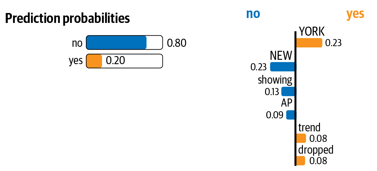
Figure 4-8. Visualization of Lime’s explanation of a classifier’s prediction
Learning with No or Less Data and Adapting to New Domains
In all the examples we’ve seen so far, we had a relatively large training dataset available for the task. However, in most real-world scenarios, such datasets are not readily available. In other cases, we may have an annotated dataset available, but it might not be large enough to train a good classifier. There can also be cases where we have a large dataset of, say, customer complaints and requests for one product suite, but we’re asked to customize our classifier to another product suite for which we have a very small amount of data (i.e., we’re adapting an existing model to a new domain). In this section, let’s discuss how to build good classification systems for these scenarios where we have no or little data or have to adapt to new domain training data.
No Training Data
Let’s say we’re asked to design a classifier for segregating customer complaints for our e-commerce company. The classifier is expected to automatically route customer complaint emails into a set of categories: billing, delivery, and others. If we’re fortunate, we may discover a source of large amounts of annotated data for this task within the organization in the form of a historical database of customer requests and their categories. If such a database doesn’t exist, where should we start to build our classifier?
The first step in such a scenario is creating an annotated dataset where customer complaints are mapped to the set of categories mentioned above. One way to approach this is to get customer service agents to manually label some of the complaints and use that as the training data for our ML model. Another approach is called “bootstrapping” or “weak supervision.” There can be certain patterns of information in different categories of customer requests. Perhaps billing-related requests mention variants of the word “bill,” amounts in a currency, etc. Delivery-related requests talk about shipping, delays, etc. We can get started with compiling some such patterns and using their presence or absence in a customer request to label it, thereby creating a small (perhaps noisy) annotated dataset for this classification task. From here, we can build a classifier to annotate a larger collection of data. Snorkel [30], a recent software tool developed by Stanford University, is useful for deploying weak supervision for various learning tasks, including classification. Snorkel was used to deploy weak supervision–based text classification models at industrial scale at Google [31]. They showed that weak supervision could create classifiers comparable in quality to those trained on tens of thousands of hand-labeled examples! [32] shows an example of how to use Snorkel to generate training data for text classification using a large amount of unlabeled data.
In some other scenarios where large-scale collection of data is necessary and feasible, crowdsourcing can be seen as an option to label the data. Websites like Amazon Mechanical Turk and Figure Eight provide platforms to make use of human intelligence to create high-quality training data for ML tasks. A popular example of using the wisdom of crowds to create a classification dataset is the “CAPTCHA test,” which Google uses to ask if a set of images contain a given object (e.g., “Select all images that contain a street sign”).
Less Training Data: Active Learning and Domain Adaptation
In scenarios like the one described earlier, where we collected small amounts of data using human annotations or bootstrapping, it may sometimes turn out that the amount of data is too small to build a good classification model. It’s also possible that most of the requests we collected belonged to billing and very few belonged to the other categories, resulting in a highly imbalanced dataset. Asking the agents to spend many hours doing manual annotation is not always feasible. What should we do in such scenarios?
One approach to address such problems is active learning, which is primarily about identifying which data points are more crucial to be used as training data. It helps answer the following question: if we had 1,000 data points but could get only 100 of them labeled, which 100 would we choose? What this means is that, when it comes to training data, not all data points are equal. Some data points are more important as compared to others in determining the quality of the classifier trained. Active learning converts this into a continuous process.
Using active learning for training a classifier can be described as a step-by-step process:
-
Train the classifier with the available amount of data.
-
Start using the classifier to make predictions on new data.
-
For the data points where the classifier is very unsure of its predictions, send them to human annotators for their correct classification.
-
Include these data points in the existing training data and retrain the model.
Repeat Steps 1 through 4 until a satisfactory model performance is reached.
Tools like Prodigy [33] have active learning solutions implemented for text classification and support the efficient usage of active learning to create annotated data and text classification models quickly. The basic idea behind active learning is that the data points where the model is less confident are the data points that contribute most significantly to improving the quality of the model, and therefore only those data points get labeled.
Now, imagine a scenario for our customer complaint classifier where we have a lot of historical data for a range of products. However, we’re now asked to tune it to work on a set of newer products. What’s potentially challenging in this situation? Typical text classification approaches rely on the vocabulary of the training data. Hence, they’re inherently biased toward the kind of language seen in the training data. So, if the new products are very different (e.g., the model is trained on a suite of electronic products and we’re using it for complaints on cosmetic products), the pre-trained classifiers trained on some other source data are unlikely to perform well. However, it’s also not realistic to train a new model from scratch on each product or product suite, as we’ll again run into the problem of insufficient training data. Domain adaptation is a method to address such scenarios; this is also called transfer learning. Here, we “transfer” what we learned from one domain (source) with large amounts of data to another domain (target) with less labeled data but large amounts of unlabeled data. We already saw one example of how to use BERT for text classification earlier in this chapter.
This approach for domain adaptation in text classification can be summarized as follows:
-
Start with a large, pre-trained language model trained on a large dataset of the source domain (e.g., Wikipedia data).
-
Fine-tune this model using the target language’s unlabeled data.
-
Train a classifier on the labeled target domain data by extracting feature representations from the fine-tuned language model from Step 2.
ULMFit [34] is another popular domain adaptation approach for text classification. In research experiments, it was shown that this approach matches the performance of training from scratch with 10 to 20 times more training examples and only 100 labeled examples in text classification tasks. When unlabeled data was used to fine-tune the pre-trained language model, it matched the performance of using 50 to 100 times more labeled examples when trained from scratch, on the same text classification tasks. Transfer learning methods are currently an active area of research in NLP. Their use for text classification has not yet shown dramatic improvements on standard datasets, nor are they the default solution for all classification scenarios in industry setups yet. But we can expect to see this approach yielding better and better results in the near future.
So far, we’ve seen a range of text classification methods and discussed obtaining appropriate training data and using different feature representations for training the classifiers. We also briefly touched on how to interpret the predictions made by some text classification models. Let’s now consolidate what we’ve learned so far using a small case study of building a text classifier for a real-world scenario.
Case Study: Corporate Ticketing
Let’s consider a real-world scenario and learn how we can apply some of the concepts we’ve discussed in this section. Imagine we’re asked to build a ticketing system for our organization that will track all the tickets or issues people face in the organization and route them to either internal or external agents. Figure 4-9 shows a representative screenshot for such a system; it’s a corporate ticketing system called Spoke.
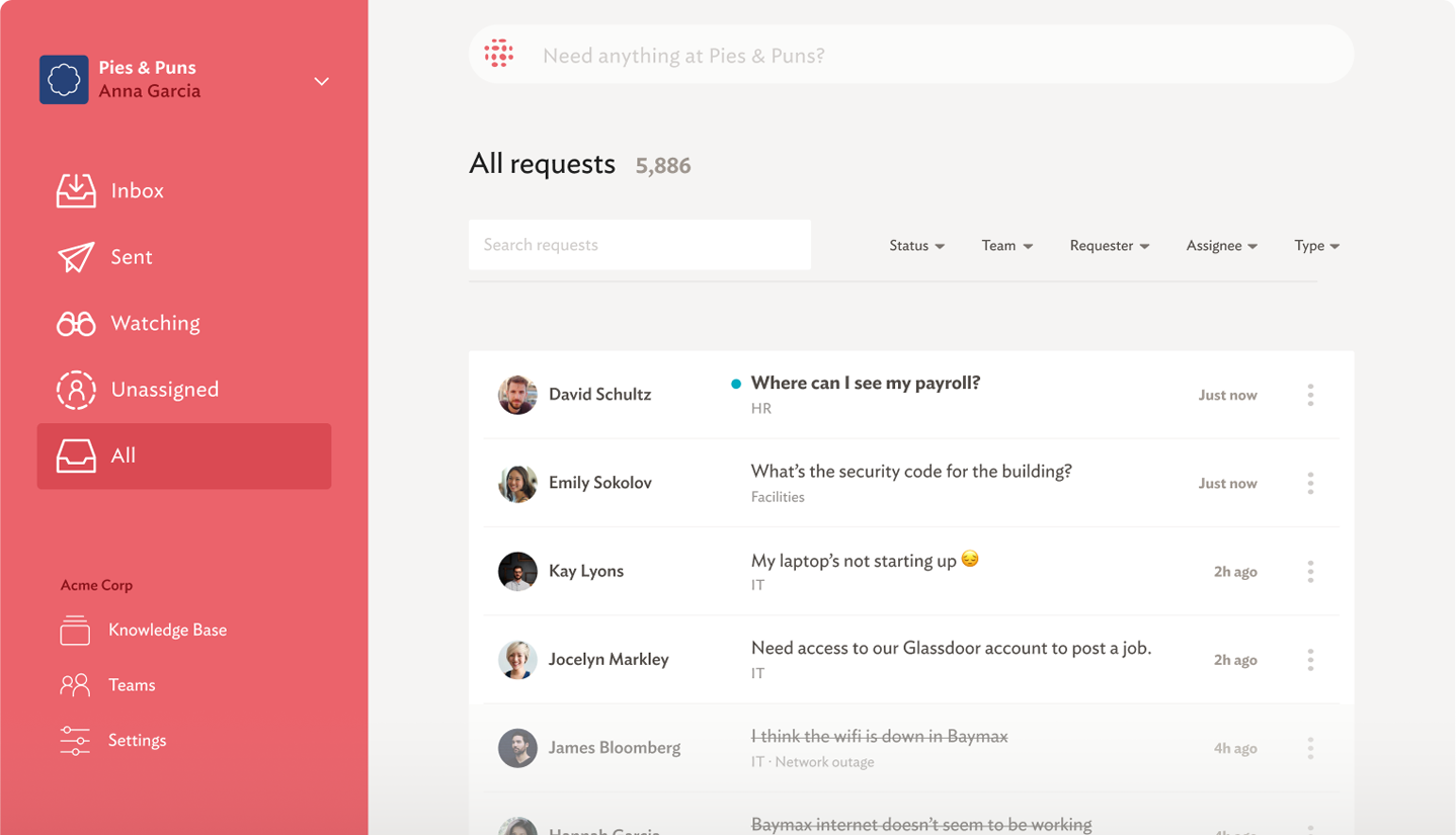
Figure 4-9. A corporate ticketing system
Now let’s say our company has recently hired a medical counsel and partnered with a hospital. So our system should also be able to pinpoint any medical-related issue and route it to the relevant people and teams. But while we have some past tickets, none of them are labeled as health related. In the absence of these labels, how will we go about building such a health issue–related classification system?
Let’s explore a couple of options:
- Use existing APIs or libraries
One option is to start with a public API or library and map its classes to what’s relevant to us. For instance, the Google APIs mentioned earlier in the chapter can classify content into over 700 categories. There are 82 categories associated with medical or health issues. These include categories like /Health/Health Conditions/Pain Management, /Health/Medical Facilities & Services/Doctors’ Offices, /Finance/Insurance/Health Insurance, etc.
While not all categories are relevant to our organization, some could be, and we can map these accordingly. For example, let’s say our company doesn’t consider substance abuse and obesity issues as relevant for medical counsel. We can ignore /Health/Substance Abuse and /Health/Health Conditions/Obesity in this API. Similarly, whether insurance should be a part of HR or referred outside can also be handled with these categories.
- Use public datasets
We can also adopt public datasets for our needs. For example, 20 Newsgroups is a popular text classification dataset, and it’s also part of the sklearn library. It has a range of topics, including sci.med. We can also use it to train a basic classifier, classifying all other topics in one category and sci.med in another.
- Utilize weak supervision
We have a history of past tickets, but they’re not labeled. So, we can consider bootstrapping a dataset out of it using the approaches described earlier in this section. For example, consider having a rule: “If the past ticket contains words like fever, diarrhea, headache, or nausea, put them in the medical counsel category.” This rule can create a small amount of data, which we can use as a starting point for our classifier.
- Active learning
We can use tools like Prodigy to conduct data collection experiments where we ask someone working at the customer service desk to look at ticket descriptions and tag them with a preset list of categories. Figure 4-10 shows an example of using Prodigy for this purpose.
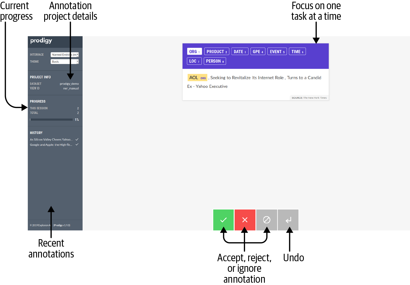
Figure 4-10. Active learning with Prodigy
- Learning from implicit and explicit feedback
Throughout the process of building, iterating, and deploying this solution, we’re getting feedback that we can use to improve our system. Explicit feedback could be when the medical counsel or hospital says explicitly that the ticket was not relevant. Implicit feedback could be extracted from other dependent variables like ticket response times and ticket response rates. All of these could be factored in to improve our model using active learning techniques.
A sample pipeline summarizing these ideas may look like what’s shown in Figure 4-11. We start with no labeled data and use either a public API or a model created with a public dataset or weak supervision as the first baseline model. Once we put this model to production, we’ll get explicit and implicit signals on where it’s working or failing. We use this information to refine our model and active learning to select the best set of instances that need to be labeled. Over time, as we collect more data, we can build more sophisticated and deeper models.
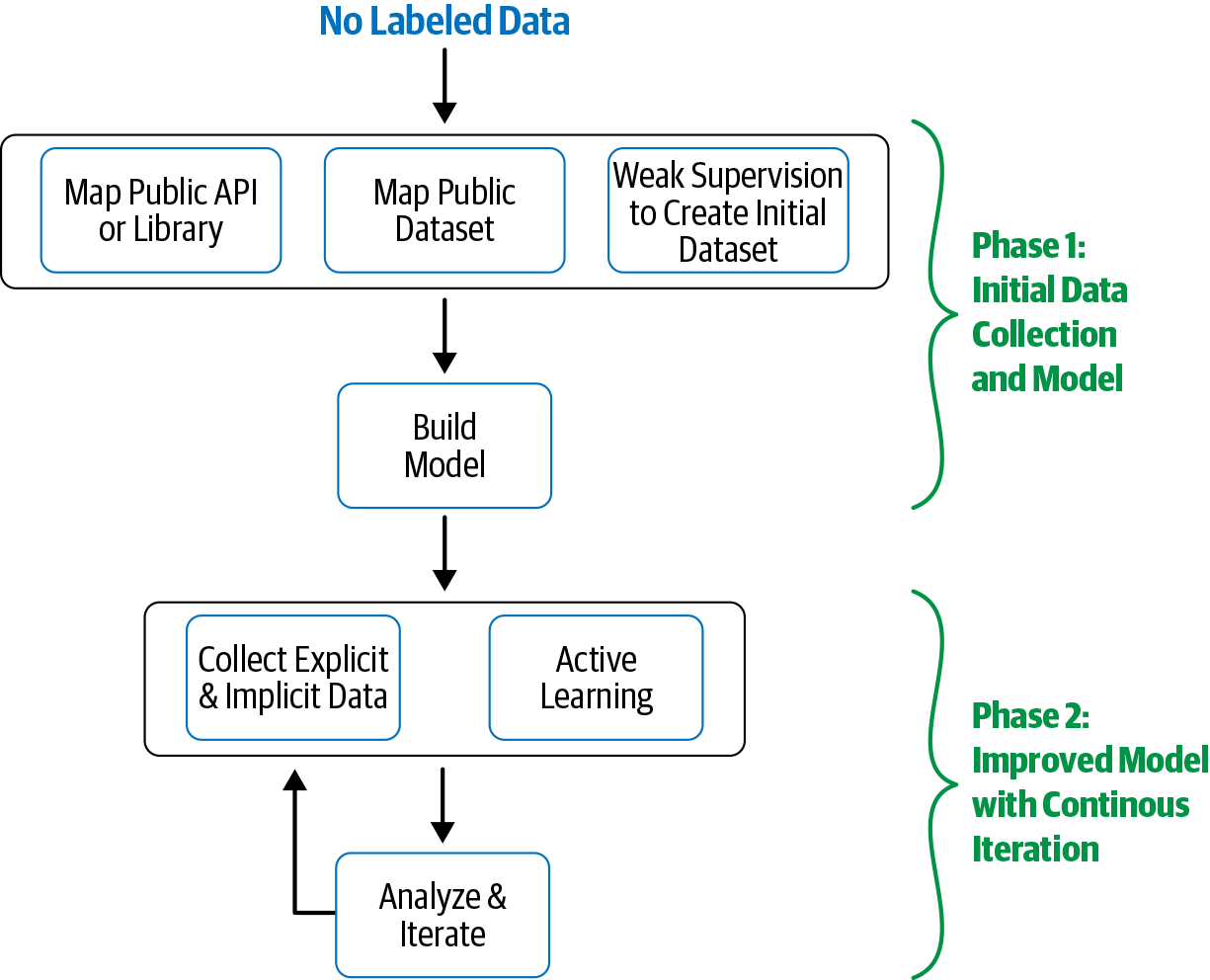
In this section, we started looking at a practical scenario of not having enough training data for building our own text classifier for our custom problem. We discussed several possible solutions to address the issue. Hopefully, this helps you foresee and prepare for some of the scenarios related to data collection and creation in your future projects related to text classification.
Practical Advice
So far, we’ve shown a range of different methods for building text classifiers and potential issues you may run into. We’d like to end this chapter with some practical advice that summarizes our observations and experience with building text classification systems in industry. Most of these are generic enough to be applied to other topics in the book as well.
- Establish strong baselines
A common fallacy is to start with a state-of-the-art algorithm. This is especially true in the current era of deep learning, where every day, new approaches/algorithms keep coming up. However, it’s always good to start with simpler approaches and try to establish strong baselines first. This is useful for three main reasons:
-
It helps us get a better understanding of the problem statement and key challenges.
-
Building a quick MVP helps us get initial feedback from end users and stakeholders.
-
A state-of-the-art research model may give us only a minor improvement compared to the baseline, but it might come with a huge amount of technical debt.
-
- Balance training data
While working with classification, it’s very important to have a balanced dataset where all categories have an equal representation. An imbalanced dataset can adversely impact the learning of the algorithm and result in a biased classifier. While we cannot always control this aspect of the training data, there are various techniques to fix class imbalance in the training data. Some of them are collecting more data, resampling (undersample from majority classes or oversample from minority classes), and weight balancing.
- Combine models and humans in the loop
In practical scenarios, it makes sense to combine the outputs of multiple classification models with handcrafted rules from domain experts to achieve the best performance for the business. In other cases, it’s practical to defer the decision to a human evaluator if the machine is not sure of its classification decision. Finally, there could also be scenarios where the learned model has to change with time and newer data. We’ll discuss some solutions for such scenarios in Chapter 11, which focuses on end-to-end systems.
- Make it work, make it better
Building a classification system is not just about building a model. For most industrial settings, building a model is often just 5% to 10% of the total project. The rest consists of gathering data, building data pipelines, deployment, testing, monitoring, etc. It is always good to build a model quickly, use it to build a system, then start improvement iterations. This helps us to quickly identify major roadblocks and the parts that need the most work, and it’s often not the modeling part.
- Use the wisdom of many
Every text classification algorithm has its own strengths and weaknesses. There is no single algorithm that always works well. One way to circumvent this is via ensembling: training multiple classifiers. The data is passed through every classifier, and the predictions generated are combined (e.g., majority voting) to arrive at a final class prediction. An interested reader can look at the work of Dong et al. [35, 36] for a deep dive into ensemble methods for text classification.
Wrapping Up
In this chapter, we saw how to address the problem of text classification from multiple viewpoints. We discussed how to identify a classification problem, tackle the various stages in a text classification pipeline, collect data to create relevant datasets, use different feature representations, and train several classification algorithms. With this, we hope you’re now well-equipped and ready to solve text classification problems for your use case and scenario and understand how to use existing solutions, build our own classifiers using various methods, and tackle the roadblocks you may face in the process. We focused on only one aspect of building text classification systems in industry applications: building the model. Issues related to the end-to-end deployment of NLP systems will be dealt with in Chapter 11. In the next chapter, we’ll use some of the ideas we learned here to tackle a related but different NLP problem: information extraction.
Footnotes
i There are other such pre-trained embeddings available. Our choice in this case is arbitrary.
References
[1] United States Postal Service. The United States Postal Service: An American History, 57–60. ISBN: 978-0-96309-524-4. Last accessed June 15, 2020.
[2] Gupta, Anuj, Saurabh Arora, Satyam Saxena, and Navaneethan Santhanam. “Noise reduction and smart ticketing for social media-based communication systems.” US Patent Application 20190026653, filed January 24, 2019.
[3] Spasojevic, Nemanja and Adithya Rao. “Identifying Actionable Messages on Social Media.” 2015 IEEE International Conference on Big Data: 2273–2281.
[4] CLPSYCH: Computational Linguistics and Clinical Psychology Workshop. Shared Tasks 2019.
[5] Google Cloud. “Natural Language”. Last accessed June 15, 2020.
[6] Amazon Comprehend. Last accessed June 15, 2020.
[7] Azure Cognitive Services. Last accessed June 15, 2020.
[8] Iderhoff, Nicolas. nlp-datasets: Alphabetical list of free/public domain datasets with text data for use in Natural Language Processing (NLP), (GitHub repo). Last accessed June 15, 2020.
[9] Kaggle. “Sentiment Analysis: Emotion in Text”. Last accessed June 15, 2020.
[10] UC Irvine Machine Learning Repository. A collection of repositories for machine learning. Last accessed June 15, 2020.
[11] Google. “Dataset Search”. Last accessed June 15, 2020.
[12] Jurafsky, Dan and James H. Martin. Speech and Language Processing, Third Edition (Draft), 2018.
[13] Lemaître, Guillaume, Fernando Nogueira, and Christos K. Aridas. “Imbalanced-learn: A Python Toolbox to Tackle the Curse of Imbalanced Datasets in Machine Learning”. The Journal of Machine Learning Research 18.1 (2017): 559–563.
[14] For a detailed mathematical description of logistic regression, refer to Chapter 5 in [12].
[15] Google. Pre-trained word2vec model. Last accessed June 15, 2020.
[16] Bojanowski, Piotr, Edouard Grave, Armand Joulin, and Tomas Mikolov. “Enriching Word Vectors with Subword Information.” Transactions of the Association for Computational Linguistics 5 (2017): 135–146.
[17] Joulin, Armand, Edouard Grave, Piotr Bojanowski, and Tomas Mikolov. “Bag of Tricks for Efficient Text Classification”. (2016).
[18] Ramesh, Sree Harsha. torchDatasets, (GitHub repo). Last accessed June 15, 2020.
[19] Joulin, Armand, Edouard Grave, Piotr Bojanowski, Matthijs Douze, Hérve Jégou, and Tomas Mikolov. “Fasttext.zip: Compressing text classification models”. (2016).
[20] For older Doc2vec versions, there are some pre-trained models; e.g., https://oreil.ly/kt0U0 (last accessed June 15, 2020).
[21] Natural Language Toolkit. “NLTK 3.5 documentation”. Last accessed June 15, 2020.
[22] Lau, Jey Han and Timothy Baldwin. “An Empirical Evaluation of doc2vec with Practical Insights into Document Embedding Generation”. (2016).
[23] Stanford Artificial Intelligence Laboratory. “Large Movie Review Dataset”. Last accessed June 15, 2020.
[24] Goodfellow, Ian, Yoshua Bengio, and Aaron Courville. Deep Learning. Cambridge: MIT Press, 2016. ISBN: 978-0-26203-561-3
[25] Goldberg, Yoav. “Neural Network Methods for Natural Language Processing.” Synthesis Lectures on Human Language Technologies 10.1 (2017): 1–309.
[26] Ribeiro, Marco Tulio, Sameer Singh, and Carlos Guestrin. “‘Why Should I Trust You?’ Explaining the Predictions of Any Classifier.” Proceedings of the 22nd ACM SIGKDD International Conference on Knowledge Discovery and Data Mining (2016): 1135–1144.
[27] Lundberg, Scott M. and Su-In Lee. “A Unified Approach to Interpreting Model Predictions.” Advances in Neural Information Processing Systems 30 (NIPS 2017): 4765–4774.
[28] Marco Tulio Correia Ribeiro. Lime: Explaining the predictions of any machine learning classifier, (GitHub repo). Last accessed June 15, 2020.
[29] Lundberg, Scott. shap: A game theoretic approach to explain the output of any machine learning model, (GitHub repo).
[30] Snorkel. “Programmatically Building and Managing Training Data”. Last accessed June 15, 2020.
[31] Bach, Stephen H., Daniel Rodriguez, Yintao Liu, Chong Luo, Haidong Shao, Cassandra Xia, Souvik Sen et al. “Snorkel DryBell: A Case Study in Deploying Weak Supervision at Industrial Scale”. (2018).
[32] Snorkel. “Snorkel Intro Tutorial: Data Labeling”. Last accessed June 15, 2020.
[33] Prodigy. Last accessed June 15, 2020.
[34] Fast.ai. “Introducing state of the art text classification with universal language models”. Last accessed June 15, 2020.
[35] Dong, Yan-Shi and Ke-Song Han. “A comparison of several ensemble methods for text categorization.” IEEE International Conference on Services Computing (2004): 419–422.
[36] Caruana, Rich, Alexandru Niculescu-Mizil, Geoff Crew, and Alex Ksikes. “Ensemble Selection from Libraries of Models.” Proceedings of the Twenty-First International Conference on Machine Learning (2004): 18.
Get Practical Natural Language Processing now with the O’Reilly learning platform.
O’Reilly members experience books, live events, courses curated by job role, and more from O’Reilly and nearly 200 top publishers.

