Predictive Control of Power Converters and Electrical Drives

5.5 Implementation

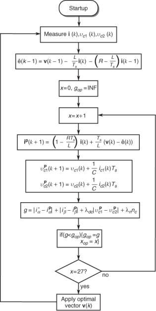
The control strategy was implemented based on a dSPACE DS1104 rapid prototyping system and MATLAB^® and Simulink^® installed on a host PC. The sampling period used with the predictive strategy was T_s = 100 μs, or a 10 kHz sampling frequency. The predictive algorithm implemented with the control platform based on the dSPACE DS1104 is explained in a flow diagram presented in Figure 5.8. The control loop begins sampling the required signals. Then, the algorithm estimates the active component of the load by means of (5.18) and initializes the value of g_op, a variable that will contain the value of the lower cost function evaluated by the algorithm so far. Then the strategy enters a loop where, for each possible switching state, the cost function (5.19) is evaluated considering current and voltage predictions obtained from (5.17), (5.11), and (5.12), respectively. If, for a given switching state, the evaluated cost function g happens to be lower than g_op, that lower value is stored as g_op and the switching state number is stored as j_op. The loop ends when all 27 switching states have been evaluated. The state that produces the optimal value of g (minimal) is identified by variable j_op and will be applied to the converter during the next sampling interval, starting the control algorithm again.

Figure 5.8 Flow diagram of the implemented control algorithm

5.5.1 Reduction ...