Reinforcement Learning

Chapter 1. Why Reinforcement Learning?

How do humans learn? This deceivingly simple question has baffled thinkers for millennia. The Greek philosopher Plato and his student Aristotle asked themselves: are truth and knowledge found within us (rationalism) or are they experienced (empiricism)? Even today, 2,500 years later, humans are still trying to answer this perpetual question.

If humans already knew everything, then they would not need to experience any more of life. Humans could spend the rest of their time on Earth improving lives by making good decisions and pondering big questions like “Where are my keys?” and “Did I lock the front door?” But how do humans gain that knowledge in the first place? You can teach knowledge. And higher levels of average education lead to a better society. But you cannot teach everything. Both in the classroom and in life, the student must experience.

Young children inspire this process. They need to experience a range of situations and outcomes. In the long term, they begin to seek rewarding experiences and avoid detrimental ones (you hope). They actively make decisions and assess the results. But a child’s life is puzzling and the rewards are often misleading. The immediate reward of climbing into a cupboard and eating a cookie is great, but the punishment is greater.

Learning by reinforcement combines two tasks. The first is exploring new situations. The second is using that experience to make better decisions. Given time, this results in a plan to achieve a task. For example, a child learns to walk, after standing up, by leaning forward and falling into the arms of a loving parent. But this is only after many hours of hand holding, wobbles, and falls. Eventually, the baby’s leg muscles operate in unison using a multistep strategy that tells them what to move when. You can’t teach every plan that the child will ever need, so instead life provides a framework that allows them a way to learn.

This book shows how you can perform the reinforcement process inside a computer. But why do this? It enables a machine to learn, by itself. To paraphrase my wife’s favorite TV show: you are providing the machine the capability to seek out new experiences, to boldly go where no machine has gone before.

This chapter presents an introduction to learning by reinforcement. (I defer a formal definition of reinforcement learning until Chapter 2.) First, I describe why engineers need this and why now. By the end of the chapter you will know which industries can use reinforcement learning and will develop your first mathematical model. You will also get an overview of the types of algorithms you will encounter later in the book.

Note

I use the word engineer throughout this book to talk abstractly about anyone who uses their skill to design a solution to solve a problem. So I mean software engineers, data engineers, data scientists, researchers, and so on.

Why Now?

Two reasons have precipitated the need and ability to perform reinforcement learning: access to large amounts of data and faster data processing speeds.

Up to the year 2000, human knowledge was stored on analog devices like books, newspapers, and magnetic tapes. If you compressed this knowledge, then in 1993 you would have needed 15.8 exabytes of space (one exabyte is one billion gigabytes). In 2018 that had increased to 33 zettabytes (one zettabyte is one thousand billion gigabytes).¹ Cloud vendors even have to resort to shipping container-sized hard disk drives to upload large amounts of data.²

You also need the necessary computational power to analyze all that data. To show this, consider the case of one of the earliest reinforcement learning implementations.

In 1947, Dietrich Prinz worked for Ferranti in Manchester, UK. There he helped to design and build the first production version of the Manchester computer called the Ferranti Mark 1.³ He learned to program the Mark 1 under the tutelage of Alan Turing and Cicely Popplewell. Influenced by Turing’s paper on the subject, in 1952 Prinz released a chess program that could solve a single set of problems called “mate-in-2.” These are puzzles where you pick the two moves that cause a checkmate in chess. Prinz’s algorithm exhaustively searched through all possible positions to generate a solution in 15—20 minutes, on average. This is an implementation of the Monte Carlo algorithm described in Chapter 2. Prinz came to see chess programming as “a clue to methods that could be used to deal with structural or logistical problems in other areas, through electronic computers.” He was right.⁴

The confluence of the volume of data and the increasing computational performance of the hardware meant that in around 2010 it became both possible and necessary to teach machines to learn.

Machine Learning

Note

A full summary of machine learning is outside the scope of this book. But reinforcement learning depends upon it. Read as much as you can about machine learning, especially the books I recommend in “Further Reading”.

The ubiquity of data and the availability of cheap, high-performance computation has allowed researchers to revisit the algorithms of the 1950s. They chose the name machine learning (ML), which is a misnomer, because ML is simultaneously accepted as a discipline and a set of techniques. I consider ML a child of data science, which is an overarching scientific field that investigates the data generated by phenomena. I dislike the term artificial intelligence (AI) for a similar reason; it is hard enough to define what intelligence is, let alone specify how it is achieved.

ML starts with lots of information in the form of observational data. An observation represents a collection of attributes, at a single point, that describe an entity. For example, in an election poll one observation represents the prospective vote of a single person. For a recommendation task, an observation might be a click on a particular product. Engineers use ML algorithms to interpret and make decisions upon this information.

In supervised learning, labels represent the answer to the problem, for that particular observation. The algorithm then attempts to use the information to guess the correct result. Unsupervised learning works without labels and you make decisions based upon the characteristics of the data. I always recommend that my clients at Winder Research aim for supervised learning—by paying for or running experiments to find labels, for example—because if you don’t have any ground truth, then you will find it hard to quantify performance.

The process of finding an algorithm to solve a problem is called modeling. Engineers design models to simplify and represent the underlying phenomena. They use a model to make educated guesses about new observations. For example, a model might tell you that a new customer has provided false information in their application, or it might convert your speech into text.

Given these descriptions, consider trying to teach your child how to ride a bike. What is the best way of doing this? According to the ML paradigm, you should provide lots of observations with labels. You might tell your child to watch videos of professional cyclists. Once they have seen enough videos, ignoring any protests of boredom, you might test their ability according to some arbitrary, technical success criteria. Would this work? No.

Despite ML being fundamental to many applications, some problems do not fit. A better solution, to continue the previous example, is to let your child try. Sometimes they will try and fail. Other times they will succeed. Each decision will alter their judgment. After enough tries and some guidance, they will learn strategies to maximize their own definition of success. This is the promise of learning by reinforcement, rather than by supervision.

Reinforcement Learning

Reinforcement learning (RL) tells you how to make the best decisions, sequentially, within a context, to maximize a real-life measure of success. The decision-making entity learns this through trial and error. It is not told which decisions to make, but instead it must learn by itself, by trying them. Figure 1-1 introduces the four components of RL, and Chapter 2 delves deeper.

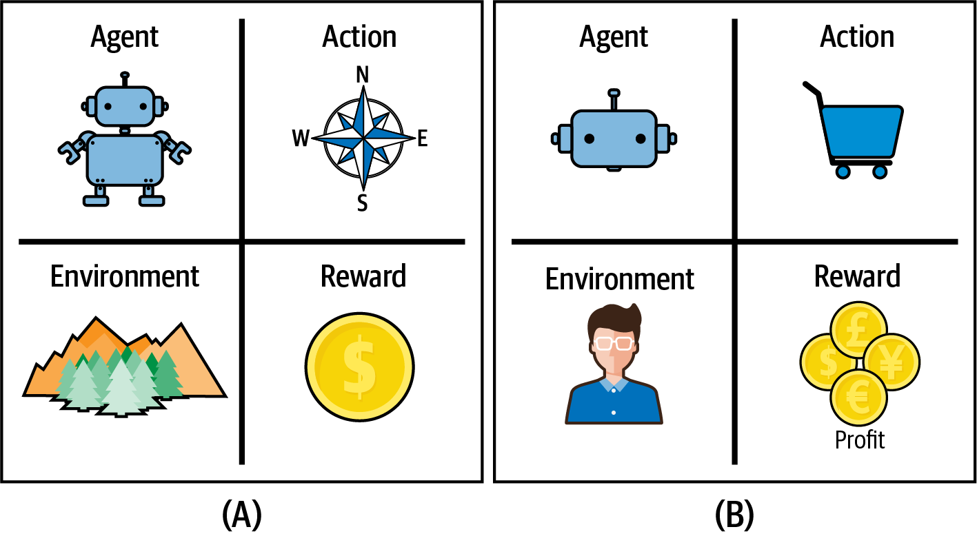
Figure 1-1. A plot of the four components required for RL: an agent, to present actions, to an environment, for the greatest reward. Example (A) shows a robot that intends to move through a maze to collect a coin. Example (B) shows an ecommerce application that automatically adds products to users’ baskets, to maximize profit.

Each decision is an action. For example, when you ride a bike the actions are the steering direction, how much to pedal, and whether to brake. If you try to automatically add items to a shopping basket, then the actions are a decision to add certain products.

The context, although it could represent any real-life situation, is often constrained to make the problem solvable. RL practitioners create an interface to interact with the environment. This could be a simulation, real life, or a combination of both. The environment accepts actions and responds with the result and a new set of observations.

The agent is the entity that makes decisions. This could be your child, some software, or a robot, for example.

The reward encodes the challenge. This feedback mechanism tells the agent which actions led to success (or failure). The reward signal is typically numeric but only needs to reinforce behavior; genetic learning strategies delete underperforming agents, rather than providing no reward, for example.

Continuing the examples, you could reward a robot for reaching a goal or the agent for adding the right product to a basket. Simple, right? But what if the robot takes three days to solve a simple maze because it spends most of the time spinning in circles? Or what if the agent starts adding all products to the basket?

This process occurs in animals, too. They must maximize the chance of survival to pass on their genes. For example, like most herbivores, moose need to eat a lot to survive. But in 2011 a moose near Gothenburg, Sweden, was found stuck in a tree after eating fermented apples.⁵ The moose reward system, which tells them to eat, has broken down because the goal is too generic. You can’t eat anything and everything to maximize your chances of survival. It’s more complicated than that.

These examples begin to highlight a major problem in RL, one that has existed since Ada Lovelace first wrote an algorithm to produce Bernoulli numbers. How do you tell a machine what you want it to do? RL agents suffer because they often optimize for the wrong thing. For now, I recommend you keep the reward as simple as you can. Problems often have a natural reward. Chapter 9 discusses this in more detail.

These four components represent a Markov decision process (MDP). You use MDPs to frame your problems, even nonengineering problems. Chapter 2 presents these ideas in more detail.

When Should You Use RL?

Some RL examples you find on the internet look forced. They take an ML example and attempt to apply RL despite the lack of a clear agent or action. Look at a few examples trying to incorporate RL into stock market prediction, for example. There is a possibility of using an automated agent to make trades, but in many examples this isn’t the focus; the focus is still on the predictive model. This is not appropriate and is best left to ML.

RL works best when decisions are sequential and actions lead to exploration in the environment. Take robotics, a classic RL application. The goal of a robot is to learn how to perform unknown tasks. You shouldn’t tell the robot how to succeed because this is either too difficult (how do you tell a robot to build a house) or you may be biased by your own experience (you are not a robot), so you don’t know the best way to move as a robot. If instead you allow the robot to explore, it can iterate toward an optimal solution. This is a good fit for RL.

Tip

You should always choose the simplest solution that solves your immediate problem to a satisfactory level.

RL’s primary advantage is that it optimizes for long-term, multistep rewards. A secondary benefit is that it is very easy to incorporate metrics used by the business. For example, advertising solutions are typically optimized to promote the best click-through rates for an individual advertisement. This is suboptimal, because viewers often see multiple advertisements and the goal is not a click, but something bigger like retention, a sign-up, or a purchase. The combination of advertisements shown, in what order, with what content, can all be optimized automatically by RL utilizing an easy-to-use goal that matches the business’ needs.

You can forgo some of the four components presented in the previous section to make development easier. If you don’t have a natural reward signal, like a robot reaching a goal, then it is possible to engineer an artificial reward. It is also common to create a simulation of an environment. You can quantize or truncate actions. But these are all compromises. A simulation can never replace real-life experience.

RL actively searches for the optimal model. You don’t have to generate a random sample and fit offline. Rapid, online learning can work wonders when it is important to maximize performance as quickly as possible. For example, in profit-based A/B tests, like deciding what marketing copy to use, you don’t want to waste time collecting a random sample if one underperforms. RL does this for free. You can learn more about how A/B testing relates to RL in Chapter 2.

Tip

In summary, RL is best suited to applications that need sequential, complex decisions and have a long-term goal (in the context of a single decision). ML might get you halfway there, but RL excels in environments with direct feedback. I have spoken to some practitioners that have used RL to replace teams of data scientists tweaking performance out of ML solutions.

RL Applications

Throughout this book I present a range of examples for two reasons. First, I want to illustrate the theoretical aspects, like how algorithms work. These examples are simple and abstract. Personally, I find that seeing examples helps me learn. I also recommend that you try to replicate the examples to help you learn. Second, I want to show how to use RL in industry.

The media has tended to focus on examples where agents defeat humans at games. They love a good story about humans becoming obsolete. And academics continue to find games useful because of the complex simulated environments. But I have decided not to talk about DeepMind’s AlphaGo Zero, a version of the agent that defeated the Go world champion, nor OpenAI Five, which beat the Dota 2 world champions, and instead focus on applications and examples across a broad range of industries. I am not saying that gaming examples are a waste of time. Gaming companies can use RL for many practical purposes, like helping them test or optimizing in-game “AIs” to maximize revenue. I am saying that I want to help you look past the hype and show you all the different places where RL is applicable. To show you what is possible, I present a broad selection of experiments that I personally find interesting:

• The field of robotics has many applications, including improving the movement and manufacturing, playing ball-in-a-cup, and flipping pancakes.⁶ Autonomous vehicles are also an active topic of research.⁷

• You can use RL to improve cloud computing. One paper optimizes applications for latency,⁸ another power efficiency/usage.⁹ Datacenter cooling, CPU cooling, and network routing are all RL applications in use today.^10,11,12

• The financial industry uses RL to make trades and to perform portfolio allocation.^13,14 And there is significant interest in optimizing pricing in real time.¹⁵

• The amount of energy used by buildings (through heating, water, light, and so on) can be significantly reduced with RL.¹⁶ And electric grids can leverage RL to deal with situations where demand is complex; homes are both producers and consumers.¹⁷

• RL is improving traffic light control and active lane management.^18,19 Smart cities also benefit.²⁰

• Recent papers suggest many applications of RL in healthcare, especially in the areas of dosing and treatment schedules.^21,22 RL can be used to design better prosthetics and prosthetic controllers.²³

• The education system and e-learning can benefit from highly individualized RL-driven curriculums.²⁴

No business sector is left untouched: gaming, technology, transport, finance, science and nature, industry, manufacturing, and civil services all have cited RL applications.

Note

I don’t want to lose you in an infinite list, so instead I refer you to the accompanying website where I have a comprehensive catalog of RL applications.

Any technology is hazardous in the wrong hands. And like the populist arguments against AI, you could interpret RL as being dangerous. I ask that as an engineer, as a human, consider what you are building. How will it affect other people? What are the risks? Does it conflict with your morals? Always justify your work to yourself. If you can’t do that, then you probably shouldn’t be doing it. The following are three more documented nefarious applications. Each one has a different ethical boundary. Where is your boundary? Which applications are acceptable to you?

• Pwnagotchi is a device powered by RL that actively scans, sniffs, and hacks WPA/WPA2 WiFi networks by decrypting handshakes.²⁵

• Researchers showed that you can train agents to evade static malware models in virus scanners.²⁶

• The US Army is developing warfare simulations to demonstrate how autonomous robots can help in the battlefield.²⁷

I discuss safety and ethics in more depth in Chapter 10.

Taxonomy of RL Approaches

Several themes have evolved throughout the development of RL. You can use these themes to group algorithms together. This book details many of these algorithms, but it helps to provide an overview now.

Model-Free or Model-Based

The first major decision that you have to make is whether you have an accurate model of the environment. Model-based algorithms use definitive knowledge of the environment they are operating in to improve learning. For example, board games often limit the moves that you can make, and you can use this knowledge to (a) constrain the algorithm so that it does not provide invalid actions and (b) improve performance by projecting forward in time (for example, if I move here and if the opponent moves there, I can win). Human-beating algorithms for games like Go and poker can take advantage of the game’s fixed rules. You and your opponent can make a limited set of moves. This limits the number of strategies the algorithms have to search through. Like expert systems, model-based solutions learn efficiently because they don’t waste time searching improper paths.^{28, 29}

Model-free algorithms can, in theory, apply to any problem. They learn strategies through interaction, absorbing any environmental rules in the process.

This is not the end of the story, however. Some algorithms can learn models of the environment at the same time as learning optimal strategies. Several new algorithms can also leverage the potential, but unknown actions of other agents (or other players). In other words, these agents can learn to counteract another agent’s strategies.

Algorithms such as these tend to blur the distinction between model-based and model-free, because ultimately you need a model of the environment somewhere. The difference is whether you can statically define it, whether you can learn it, or whether you can assume the model from the strategy.

Note

I dedicate this book to model-free algorithms because you can apply them to any industrial problem. But if you have a situation where your environment has strict, static rules, consider developing a bespoke model-based RL algorithm that is able to take advantage.

How Agents Use and Update Their Strategy

The goal of any agent is to learn a strategy that maximizes a reward. I use the word strategy, because the word is easier to understand, but the correct term is policy. Chapter 2 introduces policies in more detail.

Precisely how and when an algorithm updates the strategy is the defining factor between the majority of model-free RL algorithms. There are two key forms of strategy that dominate the performance and functionality of the agent, but they are very easy to confuse.

The first is the difference between online and offline updates to the strategy. Online agents improve their strategies using only the data they have just observed and then immediately throw it away. They don’t store or reuse old data. All RL agents need to update their strategy when they encounter a new experience to some extent, but most state-of-the-art algorithms agree that retaining and reusing past experience is useful.

Offline agents are able to learn from offline datasets or old logs. This can be a major benefit because sometimes it is difficult or expensive to interact with the real world. However, RL tends to be most useful when agents learn online, so most algorithms aim for a mix of online and offline learning.

The second, sometimes subtle, difference depends on how agents select the action defined by its strategy. On-policy agents learn to predict the reward of being in particular states after choosing actions according to the current strategy. Off-policy agents learn to predict the reward after choosing any action.

I appreciate this subtlety is difficult to understand, so let me present a quick example. Imagine you are a baby and about ready to try new food. Evolution was kind enough to provide sweet sensors on your tongue that make you feel happy, so you love your mother’s milk. An on-policy baby would attempt to learn a new policy using the current policy as a starting point. They would likely tend toward other sweet things that taste like milk. On-policy baby would have a “sweet tooth.” Off-policy baby, however, still uses the current policy as a starting point, but is allowed to explore other, possibly random choices, while still being given milk. Off-policy baby would still like sweet milk, but might also find that they like other pleasing tastes.

The distinction may seem small at this point, but this early discovery enabled the amazing RL-driven feats you see today. Most state-of-the-art algorithms are off-policy, to encourage or improve exploration. They allow for the use of a planning mechanism to direct the agent and tend to work better on tasks with delayed rewards. However, on-policy policy algorithms tend to learn quicker, because they can instantly exploit new strategies. Modern algorithms try to form a balance between these qualities for the best of both worlds.

Discrete or Continuous Actions

Actions within an environment can take many forms: you could vary the amount of torque to apply to a motor controller, decide whether to add a banana to a shopping basket, or buy millions of dollars of stock on a trade.

Some actions are binary: a stop/go road sign has precisely two classes. Other times you might have categories that you can encode into binary actions. For example, you could quantize the throttle control of a vehicle into three binary actions: none, half-power, and full power.

But often actions require more finesse. When you drive a car you rotate the steering wheel over an infinite number of angles. If you made it discrete, pain would ensue. How would you like it if your bus driver turned the steering wheel in 90-degree increments?

The weight or length of time of an action might also be important. In Super Mario Bros. the longer you hold the jump button the higher Mario jumps. You could make time part of the problem and have a continuous action that represents the amount of time to hold a button, for example. Or you could make it discrete and ensure you repeatedly poll the agent to see if it should continue to perform the action. If you can argue that the length of time of the action is decoupled from performing the action, they could be separate variables.

RL algorithms should handle both binary and continuously variable actions. But many algorithms are limited to one.

Optimization Methods

Somewhere around 14 to 16 years old, you probably learned how to solve linear equations by hand when given data and lots of paper. But the examples you worked with were probably very simple, using a single unknown variable. In the real world you will often work with hundreds, thousands, or even millions of independent variables. At this point it becomes infeasible to use the same methods you learned at school because of the computational complexity.

In general, you build models (which may or may not contain linear equations) and train them using an optimization method. RL has the same problem. You want to build an agent that is able to produce a solution given a goal. Precisely how it does this creates another fundamental theme in RL.

One way is to try as many actions as possible and record the results. In the future you can guide the agent by following the strategy that led to the best result. These are called value-based algorithms, and I introduce you to them shortly.

Another way is to maintain a model and tweak the parameters of the model to tend toward the actions that produced the best result. These are called policy-based algorithms. You can read more about them in Chapter 5.

To help you understand this, imagine a two-dimensional grid with a cliff toward the south. Your task is to design a robot that will repeatedly test each square and learn that there is a cost associated with falling off the cliff. If you used a value-based algorithm, and if you converted the strategy into words, it would say “do not step off a cliff.” A policy-based algorithm would say “move away from the cliff.” A subtle but important difference.

Value- and policy-based algorithms are currently the most studied and therefore the most popular. But imitation-based algorithms, where you optimize the agent to mimic the actions of an expert, can work well when you are trying to incorporate human guidance. Any other algorithms that don’t fit into any of these classes may spawn new methodologies in the future.

Policy Evaluation and Improvement

Another way of interpreting how an algorithm improves its strategy is to view it in terms of policy evaluation and policy improvement, shown in Figure 1-2.

First, an agent follows a strategy (the policy) to make decisions, which generates new data that describes the state of the environment.

From this new data, the agent attempts to predict the reward from the current state of the environment; it evaluates the current policy.

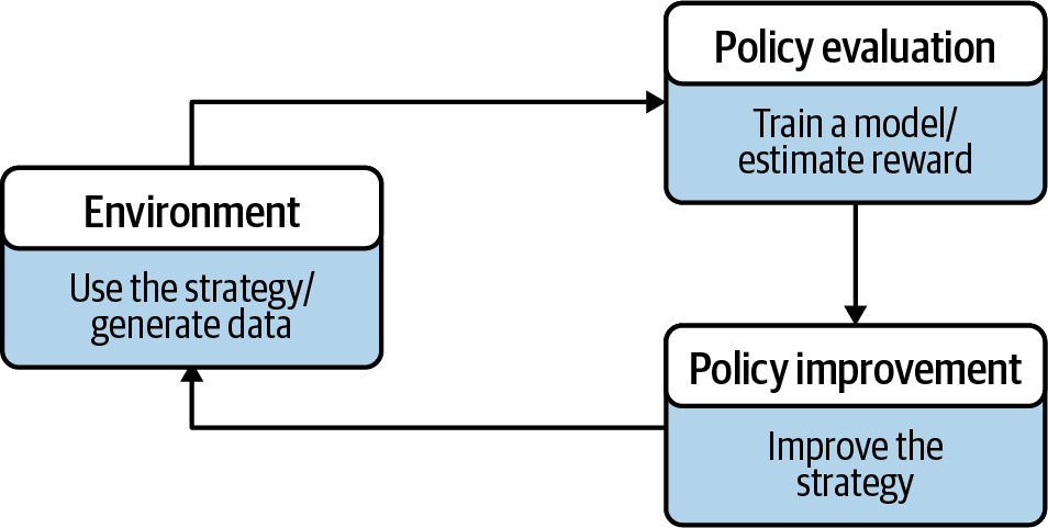
Figure 1-2. An interpretation of how algorithms update their strategy.

Next, the agent uses this prediction to decide what to do next. In general it tries to change the strategy to improve the policy. It might suggest to move to a state of higher predicted reward, or it might choose to explore more. Either way, the action is presented back to the environment and the merry-go-round starts again.

Tip

The vast majority of algorithms follow this pattern. It is such a fundamental structure that if I ever get the opportunity to rewrite this book, I would consider presenting the content in this way.

Fundamental Concepts in Reinforcement Learning

The idea of learning by reinforcement through trial and error, the fundamental basis for all RL algorithms, originated in early work on the psychology of animal learning. The celebrated Russian physiologist Ivan Pavlov first reported in 1927 that you can trigger an animal’s digestive system using stimuli that are irrelevant to the task of eating. In one famous experiment he measured the amount of saliva produced by dogs when presented with food. At the same time, he introduced a sound. After several repetitions, the dog salivated in response to the sound alone.³⁰

Sound is not a natural precursor to food, nor does it aid eating. The connection between innate reflexes, such as eye blinking or saliva generation, and new stimuli is now called classical, or Pavlovian, conditioning.

The First RL Algorithm

In 1972 Robert Rescorla and Allan Wagner found another interesting phenomenon that Pavlovian conditioning couldn’t explain. They first blew a puff of air into a rabbit’s eye, which caused it to blink. They then trained the rabbit to associate an external stimulus, a sound, with the puff of air. The rabbit blinked when it heard the sound, even if there was no puff of air. They then retrained the rabbit to blink when exposed to both a sound and a light. Again, when the rabbit heard the sound and saw the light with no puff of air, it blinked. But next, when the researchers only flashed the light, the rabbit did not blink.³¹

The rabbit had developed a hierarchy of expectations; sound and light equals blink. When the rabbit did not observe the base expectation (the sound), this blocked all subsequent conditioning. You may have experienced this sensation yourself. Occasionally you learn something so incredible, so fundamental, you might feel that any derivative beliefs are also invalid. Your lower-level conditioning has been violated and your higher-order expectations have been blocked. The result of this work was the Rescorla–Wagner model. Their research was never presented this way, but this describes a method called value estimation.

Value estimation

Imagine yourself trying to simulate the Rescorla–Wagner rabbit trial. The goal is to predict when the rabbit blinks. You can create a model of that experiment by describing the inputs and the expected output. The inputs represent the actions under your control and the output is a prediction of whether the rabbit blinks.

You can represent the inputs as a vector $s=(s_0,s_1,...,s_{n-1})$ where $s_i=1$ if the ith stimulus is present in a trial and zero otherwise. These are binary actions.

For example, imagine that the feature $s_0$ represents the sound and $s_1$ represents the light. Then the vector $s=[0,1]$ represents the situation where the sound is not present and the light is.

You can write the estimated output as $V$, which represents the prediction of whether the rabbit blinks or not. The states are then mapped to the correct prediction using a function, $V\left(s\right)$.

Note

I have made an active decision to simplify the mathematics as much as possible, to improve readability and understanding. This means that it loses mathematical formality, like denoting an estimate with a hat, to improve readability. See the academic papers for full mathematical rigor.

Now comes the hard part: defining the mapping function. One common solution is to multiply the inputs by parameters under your control. You can alter these parameters to produce an output that depends on the inputs. These parameters are called weights and the model you have just built is linear.

The weights are defined by another vector, $w$, which is the same shape as the features. For example, the data may show that the light did not cause the rabbit to blink; it blinked only when it heard the sound. This results in a model with a weight of value 1 for the sound feature and a weight of value 0 for the light.

Formally, the function is a sum of the inputs multiplied by the weights. This operation is called a dot product. The result, which is shown in Equation 1-1, is a prediction of whether the rabbit blinks.

Equation 1-1. Value estimate

$$\begin{array}{cc}\hfill V(s,w)& \doteq w_0{s}_0+w_1{s}_1+...+w_n{s}_n\hfill \\ & =w·s=w^{⊺}s\hfill \end{array}$$

But, in general, how do you decide on the values for the weights?

Prediction error

You can use an optimization method to find the optimal parameters. The most common method is to quantify how wrong your estimate is compared to the ground truth (the correct answer). Then you can try lots of different weights to minimize the error.

The error in your prediction, $\delta$, is the difference between the actual outcome of the experiment, $E$, and the prediction (the value estimate). The prediction is based upon the current state of the environment (an observation of the rabbit), $s$, and the current weights. All variables change over time and are often denoted with the subscript $t$, but I ignore that to reduce the amount of notation. You can see this defined in Equation 1-2.

Equation 1-2. Prediction error

$$\delta \doteq E-V(s,w)$$

One way to think of Equation 1-2 is that $\delta$ is a form of surprise. If you make a prediction that the rabbit will definitely blink and it does not, then the difference between what you predicted and what happened will be large; you’d be surprised by the result.

Given a quantitative definition of surprise, how should the weights be altered? One way is to nudge the weights in proportion to the prediction error. For example, consider the situation where the expectation was that the sound (index zero) and the light (index one) had equal importance. The set of weights is $w=[1,1]$.

This time the experiment is to shine only the light, not sound. So the observed state of the experiment is $x\left(s\right)=[0,1]$. To make a prediction, $V(s,w)$, calculate the result of performing a dot product on the previous vectors. The result is 1 (blink).

When you ran your simulation, the rabbit did not blink. The value was actually 0. The value of Equation 1-2, $\delta$, is equal to −1.

Knowledge of the previous state and the prediction error helps alter the weights. Multiplying these together, the result is $\delta x\left(s\right)=[0,1]$. Adding this to the current weights yields $w=[1,0]$.

Note how the new weights would have correctly predicted the actual outcome, 0 (not blink) ($w^{⊺}x\left(s\right)={[1,0]}^{⊺}[0,1]=0$).

Weight update rule

If you have any experience with ML, you know that you should not try to jump straight to the correct, optimal result. One reason is that the experimental outcome might be noisy. Always move toward the correct result gradually and repeat the experiment multiple times. Then, due to the law of large numbers, you converge toward the best average answer, which is also the optimal one. One caveat is that this is only true if the underlying mathematics proves that convergence is inevitable; in many algorithms, like those with nonlinear approximators, it is not guaranteed.

This is formalized as an update rule for the weights. In Equation 1-3, you can control the speed at which the weights update using the hyperparameter $\alpha$, which must be between zero and one. Equation 1-3 updates the weights inline, which means that the weights in the next time step derive from the weights in the current time step. Again, I ignore the subscripts to simplify the notation.

Equation 1-3. Weight update rule

$$w\leftarrow w-\alpha \delta x\left(s\right)$$

Is RL the Same as ML?

The mathematics presented in Equation 1-1 and Equation 1-3 provide one psychological model of how animals learn. You could easily apply the same approach to software-controlled agents. But the real reason for going into such depth was to provide a mathematical warm-up exercise for the rest of the book. Here I used mathematical symbols that are used in later chapters (the original paper used different symbols and terminology from psychology).

If you ignore the mathematics for a moment, the idea of updating the weights to produce a better fit might sound familiar. You are right; this is regression from ML. The objective is to predict a numerical outcome (the total reward) from a given set of inputs (the observations). Practitioners call this the the prediction problem. In order to make good decisions, you need to be able to predict which actions are optimal.

The main thing that differentiates ML from RL is that you are giving agents the freedom of choice. This is the control part of the problem and at first glance looks like a simple addition on top of the ML prediction problem. But don’t underestimate this challenge. You might think that the best policy is to pick the action with the highest prediction. No, because there may be other states that are even more rewarding.

Control endows autonomy; super-machines can learn from their own mistakes. This skill opens a range of new opportunities. Many challenges are so complicated—teaching a robot to take pictures of a specific object, for example—that engineers have to resort to constraints, rules, and splitting the challenge into micro-problems. Similarly, I work with clients who have to retrain their models on a daily or hourly basis to incorporate new data. No more. Relinquish control and use RL.

RL algorithms attempt to balance these two concerns, exploration and exploitation, in different ways. One common difference is how algorithms alter the rate at which they explore. Some explore at a fixed rate, others set a rate that is proportional to the prediction of the value. Some even attempt the probability of attaining the maximum reward for a given state. This is discussed throughout the book.

Reward and Feedback

ML researchers have taken inspiration from neuroscience. The most commonly cited example of this is the development of the artificial neuron, the basis of neural networks and deep learning, which is a model of the constituent unit in your brain, much like how the atomic model summarizes an elemental unit of matter. RL, in particular, has been influenced by how the brain communicates.

A neurotransmitter, dopamine, is produced by special cells in the brain. It is involved in major brain processes, including motivation and learning and, therefore, decision making. It can also have negative aspects such as addiction and a range of medical disorders. Although there is still much unknown about dopamine, it is known to be fundamental in processing rewards.

Traditional theories about the presence of dopamine relied upon the reinforcing and pleasurable effect of the chemical. But studies in the early 1990s showed a number of startling facts. Researchers were able to quantitatively measure the activity of dopamine in monkeys. Their results showed that there was a background level of constant dopamine release. They then trained each monkey in a traditional conditioning task, like the one you saw in “Value estimation”, where the monkeys expected food a few minutes after they were shown a light. When the training started, there was a significant increase over background dopamine levels when the reward was given. Over time, the researchers observed that the dopamine release in the monkeys shifted toward the onset of the light. Eventually, each monkey produced a dopamine spike whenever they saw a light.³² If you excuse the leap to human experiences, I can attest that my children are more excited about the prospect of getting ice cream than actually eating the ice cream.

An even more fascinating follow-up study used the same conditioning training and observed the same dopamine spike when a monkey predicted the reward due to the conditioned stimulus. However, when the researchers showed the stimulus but did not give the monkey a reward at the expected time, there was a significant decrease in background dopamine levels. There was a negative dopamine effect (if compared to the baseline) when the monkey did not receive a reward.³³

Like in “Prediction error”, these experiences can be well modeled by a corrective process. The dopamine neurons are not signaling a reward in itself. The dopamine is the signal representing the reward prediction errors. In other words, dopamine is the brain’s $\delta$.

Delayed rewards

A reward simulates the idea of motivation in agents. What motivates you to get up in the morning? Are you instantly rewarded? Probably not. This is why delayed gratification is such an important, and difficult, life skill to master. The reward for getting out of bed in the morning, eating a healthy breakfast, working hard, and being nice to people is different for all of us.

The delayed reward problem is also difficult to solve in RL. Often an agent needs to wait a long time to observe the reward. Algorithmic tricks can help here, but fundamentally, altering the reward signal so it provides more frequent updates helps guide the agent toward the solution. Altering the reward this way is called reward shaping, but I like to think of it as reward engineering, akin to feature engineering in ML.

Related to this problem is the attribution of a reward. For example, which decisions caused you to end up in the situation you are in now? How can you know? An early decision may have made the difference between success and failure. But given all the possible states and actions in a complex system, solving this problem is difficult. In general it is only possible to say that the decisions are optimal on average, given a set of assumptions and constraints.

Hindsight

The idiom trust your gut means that you should trust your instinctive reaction when observing a new situation. These heuristic shortcuts have been learned through years of experience and generally lead to good results. Critical thinking, the process where you logically and methodically work through a problem, takes much more energy and concentration.

These two processes in the brain, often called the system 1 and 2 models, are an energy-saving mechanism. Why waste precious mental resources dealing with the tasks that you perform on a daily basis? You would find it difficult to have to consciously think about how to walk. But Alzheimer’s sufferers have to deal with this horrendously debilitating situation every day.³⁴

Researchers propose that neurological differences within the brain account for these systems.³⁵ The job of the “instinctive” part of the brain is to quickly decide upon actions. The task of the other is to audit those actions and take corrective measures if necessary.

This structure led to the development of the actor-critic family of algorithms. The actor has the responsibility of making important decisions to maximize reward. The critic is there for future planning and to correct the actor when it gets the answer wrong. This discovery was vital for many advanced RL algorithms.

Reinforcement Learning as a Discipline

RL developed as two independent disciplines up until around the 1980s. Psychology studied animal behavior. Mechanical and electrical engineers developed the theory to describe the optimal control of systems.

The term optimal control originated in the 1950s to describe how to tune a system to maintain a goal. This culminated in 1957 when Richard Bellman developed the Markov decision process (MDP), a set of requirements for a mathematically tractable environment, and dynamic programming, a method of solving MDPs.³⁶

According to one source, studies in animal behavior go back as far as the 19th century where experiments involving “groping and experimenting” were observed.³⁷ Edward Thorndike locked cats in “puzzle boxes” and timed how long it took the cats to escape.³⁸ He found that the time to escape decreased with repeated experiences, from 5 minutes down to 6 seconds. The result of this work was the “law of effect,” which is more generally known as learning by trial and error.

The term reinforcement first appeared in the translations from Pavlov’s manuscripts on conditioned reflexes in 1927. But RL was popularized by the grandfather of computing, Alan Turing, when he penned his earliest thoughts on artificial intelligence in 1948. In the following quote he is talking about how to “organize” a physical collection of electronic circuits he called “machines” into doing something practical:

This may be done simply by allowing the machine to wander at random through a sequence of situations, and applying pain stimuli when the wrong choice is made, pleasure stimuli when the right one is made. It is best also to apply pain stimuli when irrelevant choices are made. This is to prevent getting isolated in a ring of irrelevant situations. The machine is now “ready for use”.³⁹

Alan Turing (1948)

I find it remarkable how much of Turing’s work is still relevant today. In his time researchers were building robotic machines to achieve mundane tasks. One particularly ingenious researcher called William Grey Walter built a “mechanical tortoise” in 1951. In 1953 he unveiled a “tortoise” called CORA (Conditioned Reflex Analogue) that was capable of “learning” from its environment. The robot contained circuits that could simulate Pavlovian conditioning experiments. Even then, the public was fascinated with such machines that could “learn”:

In England a police whistle has two notes which sound together and make a particularly disagreeable sound. I tried to teach [CORA], therefore, that one note meant obstacle, and that the other note meant food. I tried to make this differential reflex by having two tuned circuits, one of which was associated with the appetitive response and the other with the avoidance response. It was arranged that one side of the whistle was blown before the machine touched an object so that it learned to avoid that, while the other side of the whistle was blown before it was supposed to see the light. The effect of giving both notes was almost always disastrous; it went right off into the darkness on the right-hand side of the room and hovered round there for five minutes in a sort of sulk. It became irresponsive to stimulation and ran round in circles.⁴⁰

William Grey Walter (1956)

Towards the end of the 1950s researchers’ interests were shifting away from pure trial and error learning and toward supervised learning. In fact, in the early days people used to use these two terms interchangeably. The early neural network pioneers including Frank Rosenblatt, Bernard Widrow, and Ted Hoff used the terms reward and punishment in their papers. This caused confusion because supervised, unsupervised, and RL were all used to denote the same idea.

At the same time the overselling of AI in the 1950s and 1960s caused widespread dissatisfaction at the slow progress. In 1973, the Lighthill report on the state of AI research in the UK criticized the utter failure to achieve its “grandiose objectives.”⁴¹ Based upon this report, most of the public research funding in the UK was cut and the rest of the world followed. The 1970s became known as the “AI winter” and progress stalled.

The resurgence of RL in the 1980s is acknowledged to be due to Harry Klopf declaring throughout the 1970s that the knowledge and use of key learning behaviors was being lost. He reiterated that control over the environment, to achieve some desired result, was the key to intelligent systems. Richard Sutton and Andrew Barto worked in the 1980s and 1990s to advance Klopf’s ideas to unite the fields of psychology and control theory (see “Fundamental Concepts in Reinforcement Learning”) through temporal-difference (TD) learning. In 1989 Chris Watkins integrated all previous threads of RL research and created Q-learning.

I end my very brief look at the history of RL here because the results of the next 30 years of research is the content of this book. You can learn more about the history of RL from the references in “Further Reading”.

Summary

The market research firm Gartner suggests that in the US, AI augmentation is worth trillions of dollars per year to businesses.⁴² RL has a big part to play in this market, because many of today’s business problems are strategic. From the shop floor to the C-level, businesses are full of unoptimized multistep decisions like adding items to shopping baskets or defining a go-to-market strategy. Alone, ML is suboptimal, because it has a myopic view of the problem. But the explosion of data, computational power, and improved simulations all enable software-driven, ML-powered, RL agents that can learn optimal strategies that outperform humans.

Biological processes continue to inspire RL implementations. Early psychological experiments highlighted the importance of exploration and reward. Researchers have proposed different ways of emulating learning by reinforcement, which has led to several common themes. As an engineer, you must decide which of these themes suit your problem; for example, how you optimize your RL algorithm, what form the actions take, whether the agent requires a formal planning mechanism, and whether the policy should be updated online. You will gain more experience throughout this book, and in the final chapters I will show you how to apply them. With the careful definition of actions and rewards, you can design agents to operate within environments to solve a range of industrial tasks. But first you need to learn about the algorithms that allow the agents to learn optimal policies. The main purpose of this book, then, is to teach you how they work and how to apply them.

Further Reading

• Introduction to RL:

  • There are many resources, but Sergey Levine’s is one of the best.

• History of RL:

  • Sutton, Richard S., and Andrew G. Barto. 2018. Reinforcement Learning: An Introduction. MIT Press.

  • A historical survey of RL from 1996, but still relevant today.⁴³

¹ Reinsel, David, John Gantz, and John Rydning. 2018. “The Digitization of the World from Edge to Core”. IDC.

² AWS Snowmobile is a service that allows you to use a shipping container to snail-mail your data to its datacenters.

³ “Papers of Dr Dietrich G. Prinz-Archives Hub”. n.d. Accessed 2 July 2019.

⁴ Copeland, B. Jack. 2004. The Essential Turing. Clarendon Press.

⁵ BBC News. “Drunk Swedish Elk Found in Apple Tree Near Gothenburg”. 8 September 2011.

⁶ Kormushev, Petar, et al. 2013. “Reinforcement Learning in Robotics: Applications and Real-World Challenges”. Robotics 2(3): 122–48.

⁷ Huang, Wenhui, Francesco Braghin, and Zhuo Wang. 2020. “Learning to Drive via Apprenticeship Learning and Deep Reinforcement Learning”. ArXiv:2001.03864, January.

⁸ Dutreilh, Xavier, et al. 2011. “Using Reinforcement Learning for Autonomic Resource Allocation in Clouds: Towards a Fully Automated Workflow.” ICAS 2011, The Seventh International Conference on Autonomic and Autonomous Systems, 67–74.

⁹ Liu, Ning, et al. 2017. “A Hierarchical Framework of Cloud Resource Allocation and Power Management Using Deep Reinforcement Learning”. ArXiv:1703.04221, August.

¹⁰ “DeepMind AI Reduces Google Data Centre Cooling Bill by 40%”. n.d. DeepMind. Accessed 3 July 2019.

¹¹ Das, Anup, et al. 2014. “Reinforcement Learning-Based Inter- and Intra-Application Thermal Optimization for Lifetime Improvement of Multicore Systems”. In Proceedings of the 51st Annual Design Automation Conference, 170:1–170:6. DAC ’14. New York, NY, USA: ACM.

¹² Littman, M., and J. Boyan. 2013. “A Distributed Reinforcement Learning Scheme for Network Routing”. Proceedings of the International Workshop on Applications of Neural Networks to Telecommunications. 17 June.

¹³ Wang, Haoran. 2019. “Large Scale Continuous-Time Mean-Variance Portfolio Allocation via Reinforcement Learning”. ArXiv:1907.11718, August.

¹⁴ Wang, Jingyuan, Yang Zhang, Ke Tang, Junjie Wu, and Zhang Xiong. 2019. “AlphaStock: A Buying-Winners-and-Selling-Losers Investment Strategy Using Interpretable Deep Reinforcement Attention Networks”. Proceedings of the 25th ACM SIGKDD International Conference on Knowledge Discovery & Data Mining—KDD ’19, 1900–1908.

¹⁵ Maestre, Roberto, et al. 2019. “Reinforcement Learning for Fair Dynamic Pricing.” In Intelligent Systems and Applications, edited by Kohei Arai, Supriya Kapoor, and Rahul Bhatia, 120–35. Advances in Intelligent Systems and Computing. Springer International Publishing.

¹⁶ Mason, Karl, and Santiago Grijalva. 2019. “A Review of Reinforcement Learning for Autonomous Building Energy Management”. ArXiv:1903.05196, March.

¹⁷ Rolnick, David, et al. 2019. “Tackling Climate Change with Machine Learning”. ArXiv:1906.05433, June.

¹⁸ LA, P., and S. Bhatnagar. 2011. “Reinforcement Learning With Function Approximation for Traffic Signal Control”. IEEE Transactions on Intelligent Transportation Systems 12(2): 412–21.

¹⁹ Rezaee, K., B. Abdulhai, and H. Abdelgawad. 2012. “Application of Reinforcement Learning with Continuous State Space to Ramp Metering in Real-World Conditions”. In 2012 15th International IEEE Conference on Intelligent Transportation Systems, 1590–95.

²⁰ Mohammadi, M., A. Al-Fuqaha, M. Guizani, and J. Oh. 2018. “Semisupervised Deep Reinforcement Learning in Support of IoT and Smart City Services”. IEEE Internet of Things Journal 5(2): 624–35.

²¹ Shah, Pratik. n.d. “Reinforcement Learning with Action-Derived Rewards for Chemotherapy and Clinical Trial Dosing Regimen Selection”. MIT Media Lab. Accessed 4 July 2019.

²² Liu, Ying, et al. 2017. “Deep Reinforcement Learning for Dynamic Treatment Regimes on Medical Registry Data”. Healthcare Informatics: The Business Magazine for Information and Communication Systems (August): 380–85.

²³ Mohammedalamen, Montaser, et al. 2019. “Transfer Learning for Prosthetics Using Imitation Learning”. ArXiv:1901.04772, January.

²⁴ Chi, Min, et al. 2011. “Empirically Evaluating the Application of Reinforcement Learning to the Induction of Effective and Adaptive Pedagogical Strategies”. User Modeling and User-Adapted Interaction 21(1): 137–80.

²⁵ Pwnagotchi. “Pwnagotchi: Deep Reinforcement Learning for Wifi Pwning!”.

²⁶ Anderson, Hyrum S., et al. 2018. “Learning to Evade Static PE Machine Learning Malware Models via Reinforcement Learning”. ArXiv:1801.08917, January.

²⁷ Sydney J. Freedberg, Jr. “AI & Robots Crush Foes In Army Wargame”. Breaking Defense. December 2019.

²⁸ Silver, David, et al. 2017. “Mastering the Game of Go without Human Knowledge”. Nature 550(7676): 354–59.

²⁹ Zha, Daochen, Kwei-Herng Lai, Yuanpu Cao, Songyi Huang, Ruzhe Wei, Junyu Guo, and Xia Hu. 2019. “RLCard: A Toolkit for Reinforcement Learning in Card Games”. ArXiv:1910.04376, October.

³⁰ Pavlov, I. P. 1927. Conditioned Reflexes: An Investigation of the Physiological Activity of the Cerebral Cortex. Oxford, England: Oxford Univ. Press.

³¹ Rescorla, R.A and Wagner, A.R. 1972. “A Theory of Pavlovian Conditioning: Variations in the Effectiveness of Reinforcement and Nonreinforcement.” In Classical Conditioning II: Current Research and Theory, 64–99. New York, NY: Appleton-Century-Crofts.

³² Schultz, Wolfram, Ranulfo Romo, Tomas Ljungberg, Jacques Mirenowicz, Jeffrey R. Hollerman, and Anthony Dickinson. 1995. “Reward-Related Signals Carried by Dopamine Neurons.” In Models of Information Processing in the Basal Ganglia, 233–48. Computational Neuroscience. Cambridge, MA: The MIT Press.

³³ Schultz, Wolfram, Peter Dayan, and P. Read Montague. 1997. “A Neural Substrate of Prediction and Reward”. Science 275(5306): 1593–99.

³⁴ Kahneman, Daniel. 2012. Thinking, Fast and Slow. Penguin UK.

³⁵ Takahashi, Yuji, Geoffrey Schoenbaum, and Yael Niv. 2008. “Silencing the Critics: Understanding the Effects of Cocaine Sensitization on Dorsolateral and Ventral Striatum in the Context of an Actor/Critic Model”. Frontiers in Neuroscience 2.

³⁶ Bellman, Richard. 1957. “A Markovian Decision Process.” Journal of Mathematics and Mechanics 6(5): 679–84.

³⁷ Newman, Edwin B. 1954. “Experimental Psychology”. Psychological Bulletin 51(6): 591–93.

³⁸ Thorndike, Edward L. 1898. “Animal Intelligence: An Experimental Study of the Associative Processes in Animals”. The Psychological Review: Monograph Supplements 2(4): i–109.

³⁹ Turing, A. M. 1948. “Intelligent Machinery.” In Copeland, B. Jack. 2004. The Essential Turing, 428. Clarendon Press.

⁴⁰ Grey Walter, W. (1956). Presentation: Dr. Grey Walter. In J.M. Tanner and B. Inhelder (Eds.), Discussions on Child Development: Volume 2, 21–74. London: Tavistock Publications.

⁴¹ Lighthill, J. 1973. “Artificial intelligence: A paper symposium.” Science Research Council, London.

⁴² “Gartner Says AI Augmentation Will Create $2.9 Trillion of Business Value in 2021”. n.d. Gartner. Accessed 17 August 2020.

⁴³ Kaelbling, L. P., M. L. Littman, and A. W. Moore. 1996. “Reinforcement Learning: A Survey”. ArXiv:Cs/9605103, April.