Feature Engineering for Machine Learning

Chapter 4. The Effects of Feature Scaling: From Bag-of-Words to Tf-Idf

A bag-of-words representation is simple to generate but far from perfect. If we count all words equally, then some words end up being emphasized more than we need. Recall our example of Emma and the raven from Chapter 3. We’d like a document representation that emphasizes the two main characters. The words “Emma” and “raven” both appear three times, but “the” appears a whopping eight times, “and” appears five times, and “it” and “was” both appear four times. The main characters do not stand out by simple frequency count alone. This is problematic.

It would also be nice to pick out words such as “magnificently,” “gleamed,” “intimidated,” “tentatively,” and “reigned,” because they help to set the overall tone of the paragraph. They indicate sentiment, which can be very valuable information to a data scientist. So, ideally, we’d like a representation that highlights meaningful words.

Tf-Idf : A Simple Twist on Bag-of-Words

Tf-idf is a simple twist on the bag-of-words approach. It stands for term frequency–inverse document frequency.  Instead of looking at the raw counts of each word in each document in a dataset, tf-idf looks at a normalized count where each word count is divided by the number of documents this word appears in. That is:

bow(w, d) = # times word w appears in document d

tf-idf(w, d) = bow(w, d) * N / (# documents in which word w appears)

N is the total number of documents in the dataset. The fraction N / (# documents ...) is what’s known as the inverse document frequency. If a word appears in many documents, then its inverse document frequency is close to 1. If a word appears in just a few documents, then the inverse document frequency is much higher.

Alternatively, we can take a log transform instead using the raw inverse document frequency. Logarithm turns 1 into 0, and makes large numbers (those much greater than 1) smaller. (More on this later.)

If we define tf-idf as:

tf-idf(w, d) = bow(w, d) * log (N / # documents in which word w appears)

then a word that appears in every single document will be effectively zeroed out, and a word that appears in very few documents will have an even larger count than before.

Let’s look at some pictures to understand what it’s all about. Figure 4-1 shows a simple example that contains four sentences: “it is a puppy,” “it is a cat,” “it is a kitten,” and “that is a dog and this is a pen.” We plot these sentences in the feature space of three words: “puppy,” “cat,” and “is.”

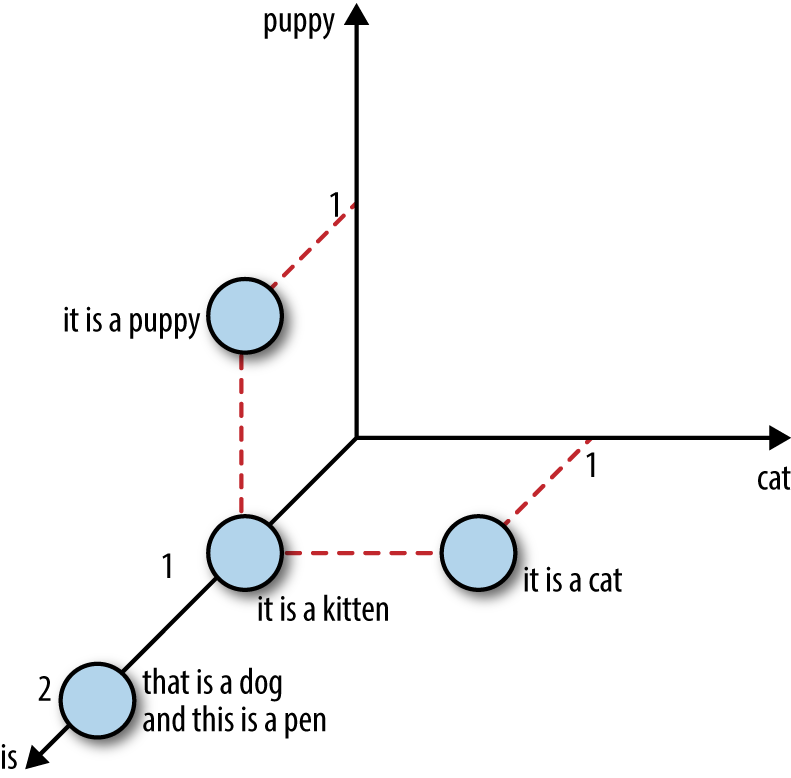
Figure 4-1. Four sentences about dogs and cats

Now let’s look at the same four sentences in tf-idf representation using the log transform for the inverse document frequency. Figure 4-2 shows the documents in feature space. Notice that the word “is” is effectively eliminated as a feature since it appears in all sentences in this dataset. Also, because they each appear in only one sentence out of the total four, the words “puppy” and “cat” are now counted higher than before (log(4) = 1.38... > 1). Thus, tf-idf makes rare words more prominent and effectively ignores common words. It is closely related to the frequency-based filtering methods in Chapter 3, but much more mathematically elegant than placing hard cutoff thresholds.

Intuition Behind Tf-Idf

Tf-idf makes rare words more prominent and effectively ignores common words.

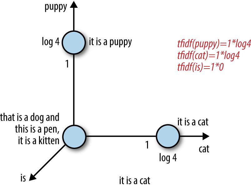
Figure 4-2. Tf-idf representation of the sentences in Figure 4-1

Putting It to the Test

Tf-idf transforms word count features through multiplication with a constant. Hence, it is an example of feature scaling, a concept introduced in Chapter 2. How well does feature scaling work in practice? Let’s compare the performance of scaled and unscaled features in a simple text classification task. Time for some code!

In Example 4-1, we revisit the Yelp reviews dataset. Round 6 of the Yelp dataset challenge contains close to 1.6 million reviews of businesses in six US cities.

Example 4-1. Loading and cleaning the Yelp reviews dataset in Python

>>> import json
>>> import pandas as pd

# Load Yelp business data
>>> biz_f = open('yelp_academic_dataset_business.json')
>>> biz_df = pd.DataFrame([json.loads(x) for x in biz_f.readlines()])
>>> biz_f.close()

# Load Yelp reviews data
>>> review_file = open('yelp_academic_dataset_review.json')
>>> review_df = pd.DataFrame([json.loads(x) for x in review_file.readlines()])
>>> review_file.close()

# Pull out only Nightlife and Restaurants businesses
>>> two_biz = biz_df[biz_df.apply(lambda x: 'Nightlife' in x['categories'] or
...                                         'Restaurants' in x['categories'], 
...                               axis=1)]

# Join with the reviews to get all reviews on the two types of business
>>> twobiz_reviews = two_biz.merge(review_df, on='business_id', how='inner')

# Trim away the features we won't use
>>> twobiz_reviews = twobiz_reviews[['business_id', 
...                                  'name', 
...                                  'stars_y', 
...                                  'text', 
...                                  'categories']]

# Create the target column--True for Nightlife businesses, and False otherwise
>>> two_biz_reviews['target'] = \
...     twobiz_reviews.apply(lambda x: 'Nightlife' in x['categories'],
...                          axis=1)

Creating a Classification Dataset

Let’s see whether we can use the reviews to categorize a business as either a restaurant or a nightlife venue. To save on training time, we can take a subset of the reviews. In this case, there is a large difference in review count between the two categories. This is called a class-imbalanced dataset. Imbalanced datasets are problematic for modeling because the model will expend most of its effort fitting to the larger class. Since we have plenty of data in both classes, a good way to resolve the problem is to downsample the larger class (restaurants) to be roughly the same size as the smaller class (nightlife). Here is an example workflow:

1. Take a random sample of 10% of nightlife reviews and 2.1% of restaurant reviews (percentages chosen so the number of examples in each class is roughly equal).

2. Create a 70/30 train-test split of this dataset. In this example, the training set ends up with 29,264 reviews, and the test set with 12,542 reviews.

3. The training data contains 46,924 unique words; this is the number of features in the bag-of-words representation.

Example 4-2 shows how we do this.

Example 4-2. Creating a balanced classification dataset

# Create a class-balanced subsample to play with
>>> nightlife = \
...   twobiz_reviews[twobiz_reviews.apply(lambda x: 'Nightlife' in x['categories'],
...                                         axis=1)]
>>> restaurants = \
...   twobiz_reviews[twobiz_reviews.apply(lambda x: 'Restaurants' in x['categories'],
...                                         axis=1)]
>>> nightlife_subset = nightlife.sample(frac=0.1, random_state=123)
>>> restaurant_subset = restaurants.sample(frac=0.021, random_state=123)
>>> combined = pd.concat([nightlife_subset, restaurant_subset])

# Split into training and test datasets
>>> training_data, test_data = modsel.train_test_split(combined, 
...                                                    train_size=0.7, 
...                                                    random_state=123)
>>> training_data.shape
(29264, 5)
>>> test_data.shape
(12542, 5)

Scaling Bag-of-Words with Tf-Idf Transformation

The goal of this experiment is to compare the effectiveness of bag-of-words, tf-idf, and ℓ² normalization for linear classification. Note that doing tf-idf then ℓ² normalization is the same as doing ℓ² normalization alone. So, we only need to test three sets of features: bag-of-words, tf-idf, and word-wise ℓ² normalization on top of bag-of-words.

In Example 4-3, we use scikit-learn’s CountVectorizer to convert the review text into a bag-of-words. All text featurization methods implicitly depend on a tokenizer, which is the module that converts a text string into a list of tokens (words). In this example, scikit-learn’s default tokenizing pattern looks for sequences of two or more alphanumeric characters. Punctuation marks are treated as token separators.

Example 4-3. Transform features

# Represent the review text as a bag-of-words 
>>> bow_transform = text.CountVectorizer()
>>> X_tr_bow = bow_transform.fit_transform(training_data['text'])
>>> X_te_bow = bow_transform.transform(test_data['text'])
>>> len(bow_transform.vocabulary_)
46924

>>> y_tr = training_data['target']
>>> y_te = test_data['target']

# Create the tf-idf representation using the bag-of-words matrix
>>> tfidf_trfm = text.TfidfTransformer(norm=None)
>>> X_tr_tfidf = tfidf_trfm.fit_transform(X_tr_bow)
>>> X_te_tfidf = tfidf_trfm.transform(X_te_bow)

# Just for kicks, l2-normalize the bag-of-words representation
>>> X_tr_l2 = preproc.normalize(X_tr_bow, axis=0)
>>> X_te_l2 = preproc.normalize(X_te_bow, axis=0)

Feature Scaling on the Test Set

A subtle point about feature scaling is that it requires knowing feature statistics that we most likely do not know in practice, such as the mean, variance, document frequency, ℓ² norm, etc. In order to compute the tf-idf representation, we have to compute the inverse document frequencies based on the training data and use these statistics to scale both the training and test data. In scikit-learn, fitting the feature transformer on the training data amounts to collecting the relevant statistics. The fitted transformer can then be applied to the test data.

When we use training statistics to scale test data, the result will look a little fuzzy. Min-max scaling on the test set no longer neatly maps to 0 and 1. ℓ² norms, mean, and variance statistics will all look a little off. This is less problematic than missing data. For instance, the test set may contain words that are not present in the training data, and we would have no document frequency to use for the new words. The common solution is to simply drop the new words in the test set. This may seem irresponsible, but the model—trained on the training set—would not know what to do with these words anyway. A slightly less hacky option would be to explicitly learn a “garbage” word and map all low-frequency words to it, even within the training set, as discussed in “Rare words”.

Classification with Logistic Regression

Logistic regression is a simple, linear classifier. Due to its simplicity, it’s often a good first classifier to try. It takes a weighted combination of the input features, and passes it through a sigmoid function, which smoothly maps any real number to a number between 0 and 1. The function transforms a real number input, x, into a number between 0 and 1. It has one set of parameters, w, which represents the slope of the increase around the midpoint, 0.5. The intercept term b denotes the input value where the function output crosses the midpoint. A logistic classifier would predict the positive class if the sigmoid output is greater than 0.5, and the negative class otherwise. By varying w and b, one can control where that change in decision occurs, and how fast the decision should respond to changing input values around that point.

Figure 4-3 illustrates the sigmoid function.

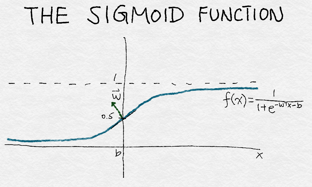
Figure 4-3. Illustration of a sigmoid function

Now let’s build some simple logistic regression classifiers on our various feature sets and see how they do (Example 4-4).

Example 4-4. Training logistic regression classifiers with default parameters

>>> def simple_logistic_classify(X_tr, y_tr, X_test, y_test, description):
...     ### Helper function to train a logistic classifier and score on test data
...     m = LogisticRegression().fit(X_tr, y_tr)
...     s = m.score(X_test, y_test)
...     print ('Test score with', description, 'features:', s)
...     return m

>>> m1 = simple_logistic_classify(X_tr_bow, y_tr, X_te_bow, y_te, 'bow')
>>> m2 = simple_logistic_classify(X_tr_l2, y_tr, X_te_l2, y_te, 'l2-normalized')
>>> m3 = simple_logistic_classify(X_tr_tfidf, y_tr, X_te_tfidf, y_te, 'tf-idf')
Test score with bow features: 0.775873066497
Test score with l2-normalized features: 0.763514590974
Test score with tf-idf features: 0.743182905438

Paradoxically, the results show that the most accurate classifier is the one using BoW features. This was unexpected. As it turns out, the reason is that the classifiers are not well “tuned,” which is a common pitfall when comparing classifiers.

Tuning Logistic Regression with Regularization

Logistic regression has a few bells and whistles. When the number of features is greater than the number of data points, the problem of finding the best model is said to be underdetermined. One way to fix this problem is by placing additional constraints on the training process. This is known as regularization, and its technical details are discussed here.

Most implementations of logistic regression allow for regularization. In order to use this functionality, one must specify a regularization parameter. Regularization parameters are hyperparameters that are not learned automatically in the model training process. Rather, they must be tuned on the problem at hand and given to the training algorithm. This process is known as hyperparameter tuning. (For details on how to evaluate machine learning models, see, e.g., Zheng [2015].) One basic method for tuning hyperparameters is called grid search: you specify a grid of hyperparameter values and the tuner programmatically searches for the best hyperparameter setting in the grid. After finding the best hyperparameter setting, you train a model on the entire training set using that setting, and use its performance on the test set as the final evaluation of this class of models.

Important: Tune Hyperparameters When Comparing Models

It’s essential to tune hyperparameters when comparing models or features. The default settings of a software package will always return a model. But unless the software performs automatic tuning under the hood, it is likely to return a suboptimal model based on suboptimal hyperparameter settings. The sensitivity of classifier performance to hyperparameter settings depends on the model and the distribution of training data. Logistic regression is relatively robust (or insensitive) to hyperparameter settings. Even so, it is necessary to find and use the right range of hyperparameters. Otherwise, the advantages of one model versus another may be solely due to tuning parameters, and will not reflect the actual behavior of the model or features.

Even the best autotuning packages still require specifying the upper and lower limits of search, and finding those limits can take a few manual tries.

In the following example, we manually set the search grid of the logistic regularization parameter to {1e-5, 0.001, 0.1, 1, 10, 100}. The upper and lower bounds took a couple of tries to narrow down. The optimal hyperparameter settings for each feature set are given in Table 4-1.

Table 4-1. Best hyperparameter settings for logistic regression on a sample of Yelp reviews of nightlife venues and restaurants

	ℓ2 regularization
BoW	0.1
ℓ2-normalized	10
Tf-idf	0.001

We also want to test whether the difference in accuracy between tf-idf and BoW is due to noise. To this end, we use k-fold cross validation to simulate having multiple statistically independent datasets. It divides the dataset into k folds. The cross validation process iterates through the folds, using all but one fold for training, and validating the results on the fold that is held out.

Estimating Variance via Resampling

Modern statistical methods assume that the underlying data comes from a random distribution. The performance measurements of models derived from data are also subject to random noise. In this situation, it is always a good idea to take the measurement not just once, but multiple times, based on datasets of comparable statistics. This gives us a confidence interval for the measurement.

k-fold cross validation is one such strategy. Resampling is another technique that generates multiple small samples from the same underlying dataset. See Zheng (2015) for more details on resampling.

The GridSearchCV function in scikit-learn runs a grid search with cross validation (see Example 4-5). Figure 4-4 shows a box-and-whiskers plot of the distribution of accuracy measurements for models trained on each of the feature sets. The middle line in the box marks the median accuracy, the box itself marks the region between the first and third quartiles, and the whiskers extend to the rest of the distribution.

Example 4-5. Tuning logistic regression hyperparameters with grid search

>>> import sklearn.model_selection as modsel

# Specify a search grid, then do a 5-fold grid search for each of the feature sets
>>> param_grid_ = {'C': [1e-5, 1e-3, 1e-1, 1e0, 1e1, 1e2]}

# Tune classifier for bag-of-words representation
>>> bow_search = modsel.GridSearchCV(LogisticRegression(), cv=5, 
...                                  param_grid=param_grid_)
>>> bow_search.fit(X_tr_bow, y_tr)

# Tune classifier for L2-normalized word vector
>>> l2_search = modsel.GridSearchCV(LogisticRegression(), cv=5,
...                                 param_grid=param_grid_)
>>> l2_search.fit(X_tr_l2, y_tr)

# Tune classifier for tf-idf
>>> tfidf_search = modsel.GridSearchCV(LogisticRegression(), cv=5,
...                                    param_grid=param_grid_)
>>> tfidf_search.fit(X_tr_tfidf, y_tr)

# Let's check out one of the grid search outputs to see how it went
>>> bow_search.cv_results_
{'mean_fit_time': array([  0.43648252,   0.94630651,  
          5.64090128,  15.31248307,  31.47010217,  42.44257565]),
'mean_score_time': array([ 0.00080056,  0.00392466,  0.00864897,  0 .00784755,  
         0.01192751,  0.0072515 ]),
'mean_test_score': array([ 0.57897075,  0.7518111 ,  0.78283898,  0.77381766,  
         0.75515992,  0.73937261]),
'mean_train_score': array([ 0.5792185 ,  0.76731652,  0.87697341,  0.94629064,  
         0.98357195,  0.99441294]),
'param_C': masked_array(data = [1e-05 0.001 0.1 1.0 10.0 100.0],
              mask = [False False False False False False],
        fill_value = ?),
'params': ({'C': 1e-05},
  {'C': 0.001},
  {'C': 0.1},
  {'C': 1.0},
  {'C': 10.0},
  {'C': 100.0}),
'rank_test_score': array([6, 4, 1, 2, 3, 5]),
'split0_test_score': array([ 0.58028698,  0.75025624,  0.7799795 ,  0.7726341 ,  
         0.75247694,  0.74086095]),
'split0_train_score': array([ 0.57923964,  0.76860316,  0.87560871,  0.94434003,  
         0.9819308 ,  0.99470312]),
'split1_test_score': array([ 0.5786776 ,  0.74628396,  0.77669571,  0.76627371,  
         0 .74867589,  0.73176149]),
'split1_train_score': array([ 0.57917218,  0.7684849 ,  0.87945837,  0.94822946,  
         0.98504976,  0.99538678]),
'split2_test_score': array([ 0.57816504,  0.75533914,  0.78472578,  0.76832394,  
         0.74799248,  0.7356911 ]),
'split2_train_score': array([ 0.57977019,  0.76613558,  0.87689548,  0.94566657,  
         0.98368288,  0.99397719]),
'split3_test_score': array([ 0.57894737,  0.75051265,  0.78332194,  0.77682843,  
         0.75768968,  0.73855092]),
'split3_train_score': array([ 0.57914745,  0.76678626,  0.87634546,  0.94558346,  
         0.98385443,  0.99474628]),
'split4_test_score': array([ 0.57877649,  0.75666439,  0.78947368,  0.78503076,  
         0.76896787,  0.75      ]),
'split4_train_score': array([ 0.57876303,  0.7665727 ,  0.87655903,  0.94763369,  
         0.98334188,  0.99325132]),
'std_fit_time': array([ 0.03874582,  0.02297261,  1.18862097,  1.83901079,  
         4.21516797,  2.93444269]),
'std_score_time': array([ 0.00160112,  0.00605009,  0.00623053,  0.00698687,  
         0.00713112,  0.00570195]),
'std_test_score': array([ 0.00070799,  0.00375907,  0.00432957,  0.00668246,  
         0.00612049]),
'std_train_score': array([ 0.00032232,  0.00102466,  0.00131222,  0.00143229,  
         0.00100223,  0.00073252])}

# Plot the cross validation results in a box-and-whiskers plot to 
# visualize and compare classifier performance
>>> search_results = pd.DataFrame.from_dict({
...                               'bow': bow_search.cv_results_['mean_test_score'],
...                               'tfidf': tfidf_search.cv_results_['mean_test_score'],
...                               'l2': l2_search.cv_results_['mean_test_score']
...                      })

# Our usual matplotlib incantations. Seaborn is used here to make
# the plot pretty.
>>> import matplotlib.pyplot as plt
>>> import seaborn as sns
>>> sns.set_style("whitegrid")

>>> ax = sns.boxplot(data=search_results, width=0.4)
>>> ax.set_ylabel('Accuracy', size=14)
>>> ax.tick_params(labelsize=14)

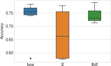
Figure 4-4. Distribution of classifier accuracy under each feature set and regularization setting—the accuracy is measured as the average accuracy from 5-fold cross validation

Table 4-2 shows the average cross validation classifier accuracy for each hyperparameter setting. The asterisk in each column denotes the highest achieved accuracy for that feature set.

Table 4-2. Average cross validation classifier accuracy scores

Regularization parameter	BoW	ℓ2-normalized	Tf-idf
0.00001	0.578971	0.575724	0.721638
0.001	0.751811	0.575724	0.788648 *
0.1	0.782839 *	0.589120	0.763566
1	0.773818	0.734247	0.741150
10	0.755160	0.776756 *	0.721467
100	0.739373	0.761106	0.712309

The result for ℓ² normalized features looks alarmingly bad in Figure 4-4. But don’t be fooled. The low accuracy numbers are due to very bad regularization parameter settings—concrete proof that suboptimal hyperparameters can lead to very wrong conclusions. If we train a model using the best hyperparameter setting for each feature set, as in Example 4-6, the accuracy scores of the different feature sets are very close.

Example 4-6. Final training and testing step to compare the different feature sets

# Train a final model on the entire training set, using the best hyperparameter 
# settings found previously. Measure accuracy on the test set.
>>> m1 = simple_logistic_classify(X_tr_bow, y_tr, X_te_bow, y_te, 'bow', 
...                               _C=bow_search.best_params_['C'])
>>> m2 = simple_logistic_classify(X_tr_l2, y_tr, X_te_l2, y_te, 'l2-normalized', 
...                               _C=l2_search.best_params_['C'])
>>> m3 = simple_logistic_classify(X_tr_tfidf, y_tr, X_te_tfidf, y_te, 'tf-idf', 
...                               _C=tfidf_search.best_params_['C'])
Test score with bow features: 0.78360708021
Test score with l2-normalized features: 0.780178599904
Test score with tf-idf features: 0.788470738319

Proper tuning improved the accuracy of all the feature sets, and all three now yield similar classification accuracy under regularized logistic regression. The accuracy score for the tf-idf model is slightly higher, but the difference is likely not statistically significant. These results are completely mystifying. If feature scaling doesn’t work better than vanilla bag-of-words, then why do it at all? Why all the hoopla if tf-idf doesn’t do anything? We’ll explore the answers to those questions in the next section.

Deep Dive: What Is Happening?

In order to understand the “why” behind the results, we have to look at how the features are being used by the model. For linear models like logistic regression, this happens through an intermediary object called the data matrix.

The data matrix contains data points represented as fixed-length flat vectors. With bag-of-words vectors, the data matrix is also known as the document-term matrix. Figure 3-1 shows a bag-of-words vector in vector form, and Figure 4-1 illustrates four bag-of-words vectors in feature space. To form a document-term matrix, simply take the document vectors, lay them out flat, and stack them on top of one another. The columns represent all possible words in the vocabulary (see Figure 4-5). Since most documents contain only a small subset of all possible words, most of the entries in this matrix are zeros; it is a sparse matrix.

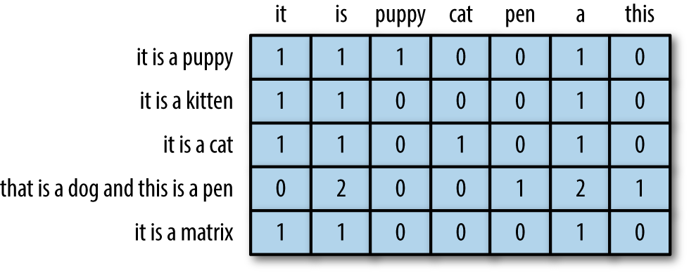
Figure 4-5. An example document-term matrix of five documents and seven words

Feature scaling methods are essentially column operations on the data matrix. In particular, tf-idf and ℓ² normalization both multiply the entire column (an n-gram feature, for example) by a constant.

Tf-Idf = Column Scaling

Tf-idf and ℓ² normalization are both column operations on the data matrix.

As discussed in Appendix A, training a linear classifier boils down to finding the best linear combination of features, which are column vectors of the data matrix. The solution space is characterized by the column space and the null space of the data matrix. The quality of the trained linear classifier directly depends upon the null space and the column space of the data matrix. A large column space means that there is little linear dependency between the features, which is generally good. The null space contains “novel” data points that cannot be formulated as linear combinations of existing data; a large null space could be problematic. (A perusal of Appendix A is highly recommended for readers who would appreciate a review on concepts such as the linear decision surface, eigen decomposition, and the fundamental subspaces of a matrix.)

How do column scaling operations affect the column space and null space of the data matrix? The answer is “Not very much.” But there is a small chance that tf-idf and ℓ² normalization could be different. We’ll look at why now.

The null space of the data matrix can be large for a couple of reasons. First, many datasets contain data points that are very similar to one another. This means the effective row space is small compared to the number of data points in the dataset. Second, the number of features can be much larger than the number of data points. Bag-of-words is particularly good at creating giant feature spaces. In our Yelp example, there are 47K features in 29K reviews in the training set. Moreover, the number of distinct words usually grows with the number of documents in the dataset, so adding more documents would not necessarily decrease the feature-to-data ratio or reduce the null space.

With bag-of-words, the column space is relatively small compared to the number of features. There could be words that appear roughly the same number of times in the same documents. This would lead to the corresponding column vectors being nearly linearly dependent, which leads to the column space being not as full rank as it could be (see Appendix A for the definition of full rank). This is called a rank deficiency. (Much like how animals can be deficient in vitamins and minerals, matrices can be deficient in rank, and the output space will not be as fluffy as it should.)

Rank-deficient row space and column space lead to the model being overly provisioned for the problem. The linear model outfits a weight parameter for each feature in the dataset. If the row and column spaces were full rank,¹ then the model would allow us to generate any target vector in the output space. When they are rank deficient, the model has more degrees of freedom than it needs. This makes it harder to pin down a solution.

Can feature scaling solve the rank deficiency problem of the data matrix? Let’s take a look.

The column space is defined as the linear combination of all column vectors (boldface indicates a vector): a₁v₁ + a₂v₂ + ... + a_nv_n. Feature scaling replaces a column vector with a constant multiple, say ${\widetilde{𝐯}}_1=c{𝐯}_{\mathbf{1}}$. But we can still generate the original linear combination by just replacing a₁ with ${\tilde{a}}_1=a_1/c$. It appears that feature scaling does not change the rank of the column space. Similarly, feature scaling does not affect the rank of the null space, because one can counteract the scaled feature column by reverse scaling the corresponding entry in the weight vector.

However, as usual, there is one catch. If the scalar is 0, then there is no way to recover the original linear combination; v₁ is gone. If that vector is linearly independent from all the other columns, then we’ve effectively shrunk the column space and enlarged the null space.

If that vector is not correlated with the target output, then this is effectively pruning away noisy signals, which is a good thing. This turns out to be the key difference between tf-idf and ℓ² normalization. ℓ² normalization would never compute a norm of zero, unless the vector contains all zeros. If the vector is close to zero, then its norm is also close to zero. Dividing by the small norm would accentuate the vector and make it longer.

Tf-idf, on the other hand, can generate scaling factors that are close to zero, as shown in Figure 4-2. This happens when the word is present in a large number of documents in the training set. Such a word is likely not strongly correlated with the target vector. Pruning it away allows the solver to focus on the other directions in the column space and find better solutions (although the improvement in accuracy will probably not be huge, because there are typically few noisy directions that are prunable in this way).

Where feature scaling—both ℓ² and tf-idf—does have a telling effect is on the convergence speed of the solver. This is a sign that the data matrix now has a much smaller condition number (the ratio between the largest and smallest singular values—see Appendix A for a full discussion of these terms). In fact, ℓ² normalization makes the condition number nearly 1. But it’s not the case that the better the condition number, the better the solution. During this experiment, ℓ² normalization converged much faster than either BoW or tf-idf. But it is also more sensitive to overfitting: it requires much more regularization and is more sensitive to the number of iterations during optimization.

Summary

In this chapter, we used tf-idf as an entry point into a detailed analysis of how feature transformations can affect the model (or not). Tf-idf is an example of feature scaling, so we contrasted its performance with that of another feature scaling method—ℓ² normalization.

The results were not as one might have expected. Tf-idf and ℓ² normalization do not improve the final classifier’s accuracy above plain bag-of-words. After acquiring some statistical modeling and linear algebra chops, we realize why: neither of them changes the column space of the data matrix.

One small difference between the two is that tf-idf can “stretch” the word count as well as “compress” it. In other words, it makes some counts bigger, and others close to zero. Therefore, tf-idf could altogether eliminate uninformative words.

Along the way, we also discovered another effect of feature scaling: it improves the condition number of the data matrix, making linear models much faster to train. Both ℓ² normalization and tf-idf have this effect.

To summarize, the lesson is: the right feature scaling can be helpful for classification. The right scaling accentuates the informative words and downweights the common words. It can also improve the condition number of the data matrix. The right scaling is not necessarily uniform column scaling.

This story is a wonderful illustration of the difficulty of analyzing the effects of feature engineering in the general case. Changing the features affects the training process and the models that ensue. Linear models are the simplest models to understand, yet it still takes very careful experimentation methodology and a lot of deep mathematical knowledge to tease apart the theoretical and practical impacts. This would be mostly impossible with more complicated models or feature transformations.

Bibliography

Zheng, Alice. Evaluating Machine Learning Models. Sebastopol, CA: O’Reilly Media, 2015.

¹ Strictly speaking, the row space and column space for a rectangular matrix cannot both be full rank. The maximum rank for both subspaces is the smaller of m (the number of rows) and n (the number of columns).