Chapter 4. Controllers
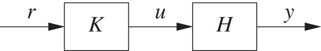
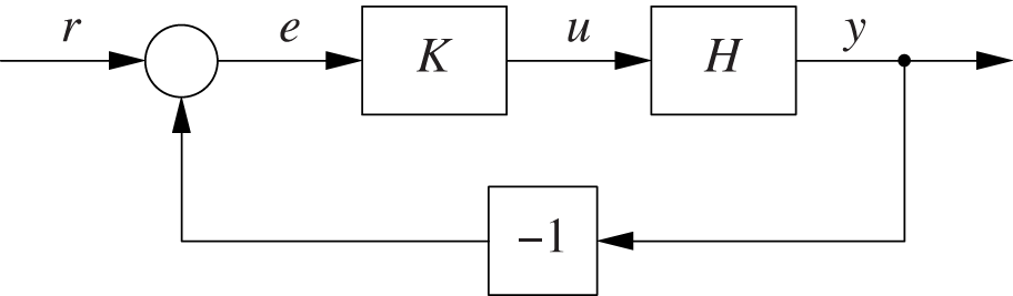
The purpose of a controller is to produce a signal that is suitable as input to the controlled plant or process. Controllers occur in both open-loop configurations (Figure 4-1) and closed-loop configurations (Figure 4-2).
The need for a controller—simply to perform numerical transformations—becomes apparent if we consider some examples. In the case of the heated vessel, the controller input will be a temperature value, but the input to the heating element itself will be a voltage, so if nothing else we need to transform units and numerical values. In the case of the read-through cache, the controller input is a hit rate and so, by construction, a number between 0 and 1 in magnitude. In contrast, the size of the cache is always positive and possibly quite large (hundreds or thousands of elements). Again, there is (at least) a need to perform a transformation of the numerical values.
Beyond the common need to transform numerical values, open-loop (feedforward) and closed-loop (feedback) configurations put different demands on a controller. In the open-loop case, the controller must be relatively “smart” in order to compensate for the complexities of the plant and its environment. By contrast, controllers used in closed loops can be extremely simple because of the self-correcting effect of the feedback path. Feedback systems trade increased complexity in overall loop architecture for a simpler controller.
Although any component that transforms an input to an output can be used as a controller in a feedback loop, only two types of controller are encountered frequently: the on/off controller and the three-term (or PID) controller. Both can be used in a feedback loop to transform their input (namely the tracking error) into a signal that is suitable as input to the controlled plant.
Block Diagrams
The structure of a control loop is easily visualized in a block diagram (see Figure 4-1 and Figure 4-2). Block diagrams consist of only three elements as follows.
The takeoff point for a signal is sometimes indicated by a small filled dot (as for the y signal in the extreme right of the closed-loop diagram in Figure 4-2). The box labeled –1 has the effect of changing the sign of its input.
There exists a collection of rules (block-diagram algebra) for manipulating block diagrams. These rules make it possible to transform and simplify diagrams purely graphically—that is, without recourse to analytic expressions—while maintaining their correct logical meaning (see Chapter 21).
On/Off Control
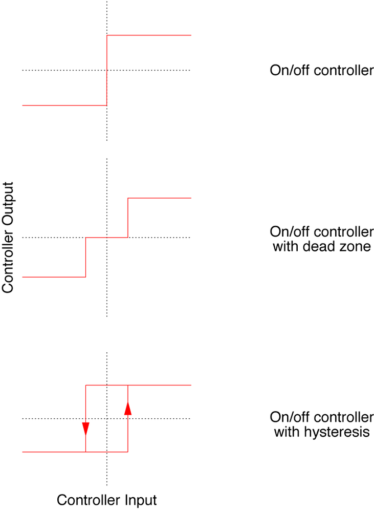
The simplest type of controller consists of nothing more than a plain on/off switch: whenever the tracking error is positive (that is, when the plant output is below the desired setpoint), the plant is being “turned on full”; whenever the tracking error is negative, the plant is being turned off. Such controllers are sometimes known as “bang-bang controllers.” See Figure 4-3.
Although deceptively simple, this control strategy has serious drawbacks that make it unsuitable for many practical applications. The main problem is that the system never settles down to a steady state; instead, it oscillates constantly and rapidly between its two extreme states. Think of a car with cruise control (which is a feedback system designed to maintain a constant speed) operating this way: instead of maintaining a steady 65 mph, an on/off cruise control would open up the throttle full whenever the speed falls even a fraction below the reference speed, only to return the engine to idle as soon as the speed exceeds the setpoint again. Such operation would be hard on the engine, the transmission, and the suspension—not to mention the passengers!
We can improve on/off controllers by augmenting them with a strategy to inhibit such rapid control oscillation. This can be done either by introducing a dead zone or by employing hysteresis. With a dead zone, the controller will not send a signal to the plant unless the tracking error exceeds some threshold value. When using hysteresis, the controller maintains the same corrective action while the tracking error switches from positive to negative (or vice versa), again until some threshold is exceeded.
Proportional Control
It is a major step forward to let the magnitude of the corrective action depend on the magnitude of the error. This has the effect that a small error will lead to only a small adjustment, whereas a larger error will result in a greater corrective action.
The simplest way to achieve this effect is to let the controller output be proportional to the tracking error:

where kp, the controller gain, is a positive constant.
Why Proportional Control Is Not Enough
Strictly proportional controllers respond to tracking errors—in particular, to changes in the tracking error—with a corrective action in the correct direction; but in general they are insufficient to eliminate tracking errors in the steady state entirely. When using a strictly proportional controller, the system output y will always be less than the desired setpoint value r, a phenomenon known as proportional droop.
The reason is that a proportional controller, by construction, can produce a nonzero output only if it receives a nonzero input. If the tracking error vanishes, then the proportional controller will no longer produce an output signal. But most systems we wish to control will require a nonzero input in the steady state. The consequence is that some residual error will persist if we rely on purely proportional control.
Proportional droop can be reduced by increasing the controller gain k, but increasing k by too much may lead to instability in the plant. Hence, a different method needs to be found if we want to eliminate steady-state errors. Of course, one can intentionally adjust the setpoint value to be higher than what is actually desired—so that, with the effect of proportional droop, the process output settles on the proper value (a process known as “manual reset”). But it turns out that this manual process is not even necessary because there is a controller design that can eliminate steady-state errors automatically. This brings us to the topic of integral control.
Integral Control
The answer to proportional droop—and, more generally, to (possibly small) steady-state errors—is to base the control strategy on the total accumulated error. The effect of a proportional controller is based on the momentary tracking error only. If this tracking error is small, then the proportional controller loses its effectiveness (since the resulting corrective actions will also be small). One way to “amplify” such small steady-state errors is to keep adding them up: over time, the accumulated value will provide a significant control signal. On the other hand, if the tracking error is zero, then the accumulated value will also be zero. This is the idea behind integral control.
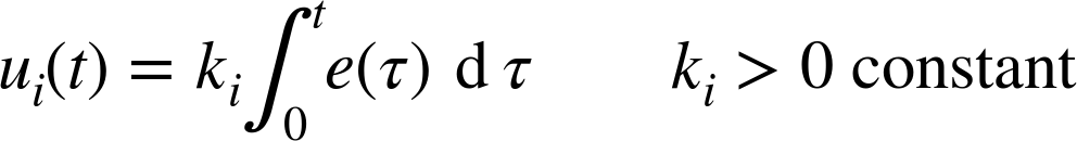
The output of an integral controller is proportional to the integral of the tracking error over time:
Bear in mind that an integral is simply a generalization of taking a sum. In a computer implementation, where time progresses in discrete steps, it becomes a sum again. An integral controller is straightforward to implement as a cumulative sum of the error values. This approach lends itself to a convenient “recursive” updating scheme:
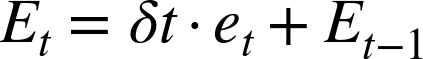
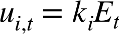
where Et is the cumulative error at time step t, ki is the integral gain, and ui,t is the output of the integral controller at time t.
This discrete updating scheme assumes that control actions are performed periodically. The factor δt is the length of time between successive control actions, expressed in the units in which we measure time. (If we measure time in seconds and make 100 control actions per second, then δt = 0.01; if we measure time in days and make one update per day, then δt = 1.) Of course, δt could be absorbed into the controller gain ki, but this would imply that if we change the update frequency (for example, by switching to two updates per day instead of one), then the controller gains also would have to change! It is better to keep things separate: δt encapsulates the time interval between successive updates, and ki independently controls the contribution of the integral term to the controller output.
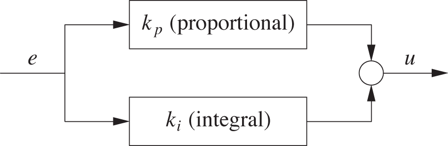
It is common to use both a proportional and an integral controller in parallel (see Figure 4-4). In fact, this particular arrangement—also known as a PI (proportional-integral) controller—is the variant most frequently used in applications.
Integral Control Changes the Dynamics
The output of an integral controller depends not only on the momentary value of the error but also on the integral (or the sum) of the observed tracking errors since the beginning of time. This dependence on past values implies that an integral controller possesses nontrivial dynamics (as discussed in Chapter 3), which may change the qualitative behavior of the entire loop.
In particular, an integral controller may introduce oscillations into a loop even if the controlled system itself is not capable of oscillations. If a positive tracking error persists, then the integral term in the controller will increase; the result will be a positive input to the plant that will persist even after the tracking error is eliminated. As a consequence, the plant output will overshoot and the tracking error will become negative. In turn, the tracking error reduces the value of the integral term.
Depending on the values chosen for the controller gains kp and ki, these oscillations may decay more or less quickly. Controller tuning is the process of finding values for these parameters that lead to the most acceptable dynamic behavior of the closed-loop system (also see Chapter 9).
Integral Control Can Generate a Constant Offset
One of the usual assumptions of control theory is that the relationship between input and output of the controlled plant is linear: y = H u. This implies that, in the steady state, there can be no nonzero output unless there is a nonzero input. In a feedback loop we try to minimize the tracking error, but we also use the tracking error as input to the controller and therefore to the plant. So how can we maintain a non-zero output when the error has been eliminated?
We can’t if we use a strictly proportional controller. That’s what “proportional droop” is all about: under proportional control, the system needs to maintain some residual, nonzero tracking error in order to produce a nonzero output. But we can drive the tracking error all the way down to zero and still maintain a nonzero plant output—provided that we include an integral term in the controller.
Here is how it works: consider (again) the heated pot on the stove. Assume that the actual temperature (that is, the system output y) is below the desired value and hence there is a nonzero, positive tracking error e = r – y. The proportional term multiplies this error by the gain to produce its control signal (up = kpe); the integral term adds the error to its internal sum of errors (E = E + e) and reports back its value (ui = kiE). In response to the combined output of the controller, more heat is supplied to the heated pot. Assume further that this additional heat succeeds in raising the temperature in the pot to the desired value. Now the tracking error is zero (e = 0) and therefore the control signal due to the proportional term is also zero (up = kp · 0 = 0). However, the internal sum of tracking errors maintained by the integral term has not changed. (It was “increased” by the current value of the tracking error, which is zero: E = E + 0 = E.) Hence the integral term continues to produce a nonzero control signal (ui = kiE), which leads to a nonzero process output. (In regards to the heated pot, the integral term ensures that a certain amount of heat continues to be supplied to the pot and thereby maintains the desired, elevated temperature in the vessel.)
Derivative Control
Finally, we can also include a derivative term in the controller. Whereas an integral term keeps track of the past, a derivative controller tries to anticipate the future. The derivative is the rate of change of some quantity. So if the derivative of the tracking error is positive, we know that the tracking error is currently growing (and vice versa). Hence we may want to apply a corrective action immediately, even if the value of the error is still small, in order to counteract the error growth—that is, before the tracking error has a chance to become large.
Therefore, we make the output of the derivative controller proportional to the derivative of the tracking error:
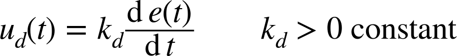
In a discrete-time computer implementation, we can approximate the derivative of e by the amount e has changed since the previous time step. A derivative controller can thus be implemented as
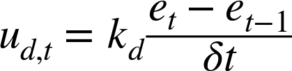
where δt is the time interval between successive updates (as for the integral term).
Like the integral controller, the derivative controller depends on past values and therefore introduces its own, nontrivial dynamics into the system.
Problems with Derivative Control
Whereas integral controllers are extremely “benevolent” and so are often used together with proportional controllers, the same cannot be said about derivative control. The problem is the potential presence of high-frequency noise in the controller input.
The noise contribution will fluctuate around zero and will thus tend to cancel itself out in an integral controller. (In other words, the integrator has a smoothing effect.) However, if we take the derivative of a signal polluted by noise, then the derivative will enhance the effect of the noise. For this reason, it will often be necessary to smooth the signal. This adds complexity (and additional nontrivial dynamics) to the controller, but it also runs the risk of defeating the purpose of having derivative control in the first place: if we oversmooth the signal, we will eliminate exactly the variations in the signal that the derivative controller was supposed to pick up!
Another problem with derivative control is the effect of sudden set-point changes. A sudden change in setpoint will lead to a very large momentary spike in the output of the derivative controller, which will be sent to the plant—an effect known as derivative kick. (In Chapter 10 we will discuss ways to avoid the derivative kick.)
Whereas proportional control is central to feedback systems, and integral control is required in order to eliminate steady-state errors, it should come as no surprise that derivative control is less widely used in practice. Studies show that as many as 95 percent of all controllers used in certain application areas are of the proportional-integral (PI) type.
The Three-Term or PID Controller
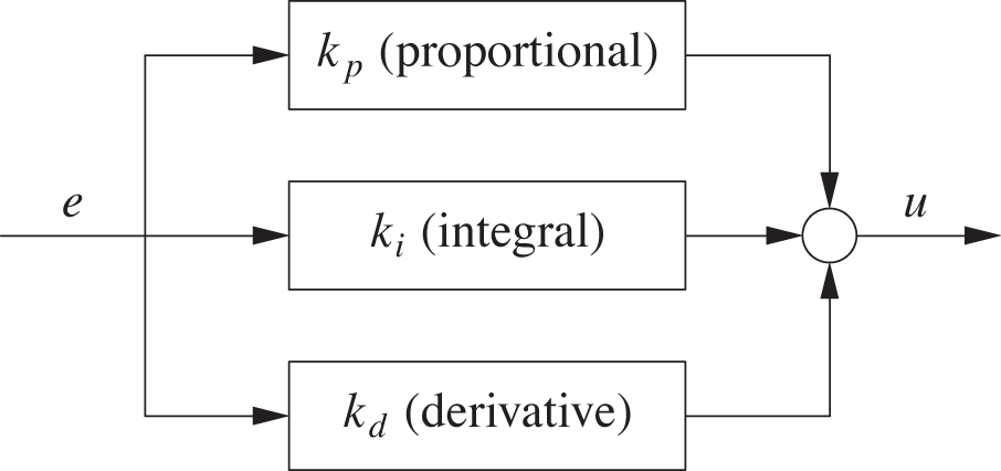
A controller including all three components (proportional, integral, and derivative) is known as a three-term or PID controller (see Figure 4-5). Its output is a combination of its three components:
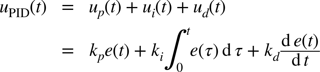
This is the form most convenient for theoretical work. In application-oriented contexts, an alternative form is often used that factors out an overall gain factor:
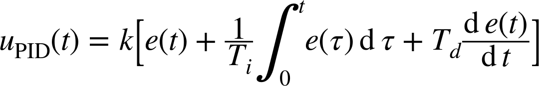
The new parameters Ti and Td both have the dimension of time. The two formulas for uPID(t) are equivalent, and their parameters are related:
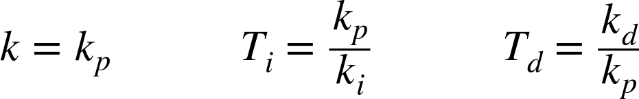
Of course, the numerical values of the parameters are different! When comparing values for controller parameters, one must not forget to establish which of the two forms they refer to.
Convention
In this book, controller gains are always nonnegative. (That is, they are zero or greater.)
We’ll pick up the study of PID controllers again in Chapter 22, by which time we will have acquired a larger set of theoretical tools.
Code to Play With
The discrete-time updating schemes for the integral and derivative terms lend themselves to straightforward computer implementations. The following class implements a three-term controller:
class PidController:
    def __init__( self, kp, ki, kd=0 ):
        self.kp, self.ki, self.kd = kp, ki, kd
        self.i = 0
        self.d = 0
        self.prev = 0

    def work( self, e ):
        self.i += DT*e
        self.d = ( e - self.prev )/DT
        self.prev = e

        return self.kp*e + self.ki*self.i + self.kd*self.d
Here the factor DT represents the step length δt, which measures the interval between successive control actions, expressed in the units in which time is measured.
This controller implementation is part of a simulation framework that can be used to explore control problems. In Chapter 12, we will discuss this framework in more detail and also introduce a better controller implementation that avoids some deficiencies of the straightforward version presented here.
Get Feedback Control for Computer Systems now with the O’Reilly learning platform.
O’Reilly members experience books, live events, courses curated by job role, and more from O’Reilly and nearly 200 top publishers.

