Chapter 4. Common Model Parameters
One of the things that makes the H2O APIs so pleasant to use is that each of the machine learning algorithms have much of their interface in common. Later chapters will look at one algorithm at a time, and show how to use them on each of our example data sets. Rather than repeat the same thing in each of those chapters, a lot of the common functionality will be here.
Note
The Python API is object-oriented, which complicates things for this chapter: most of the parameters described here are given when creating the estimator object, but a few are given when calling train() on that object. The latter ones will be pointed out as we go.
The R API (and the underlying REST API) take all parameters in one go.
Each machine learning algorithm will be introduced in its own chapter, but here are their one-line descriptions:
- Random Forest
-
An ensemble (a team) of decision trees. Parameters that apply to it are marked with
 .
. - GBM
-
Gradient Boosting Machines. Another ensemble of decision trees, but with a different approach to random forest. Indicated with
 .
. - GLM
-
Generalized Linear Models. A linear model is the idea of drawing the best straight line through data points. The generalized bit allows it to handle some nonlinearity. Indicated with
 .
. - Deep Learning
-
Multilayer neural networks, consisting of neurons in layers, and weighted connections between them. The quality improves by showing the training data over and over: each pass of the training data is called an epoch. Parameters are marked with
 .
.
Supported Metrics
H2O supports a number of metrics, ways to measure a model’s usefulness. Before we get into parameters it is worth taking a look at them because when we talk about “scoring a model” we mean evaluating on one of these metrics. The only place you specify them directly when making a model is stopping_metric, which is described later in this chapter in “Early Stopping”. But you have additional choices for sorting grids (described in “Grid Search”), or when you script custom report views.
Most only apply to either regression (predicting a continuous number) or classification (predicting a category), so they have been organized that way here.
Regression Metrics
There are two choices for early stopping:
- MSE
-
Mean Squared Error. The “squared” bit means the bigger the error, the more it is punished. If your correct answers are 2,3,4 and your algorithm guesses 1,4,3, the absolute error on each one is exactly 1, so squared error is also 1, and the MSE is 1. But if your algorithm guesses 2,3,6, the errors are 0,0,2, the squared errors are 0,0,4, and the MSE is a higher 1.333.
- deviance
-
Actually short for mean residual deviance. If the distribution is gaussian, then it is equal to MSE, and when not it usually gives a more useful estimate of error, which is why it is the default. Needs to be specified as “residual_deviance” when sorting grids.
In reports you might also see:
- RMSE
-
The square root of MSE. If your response variable units are dollars, the units of MSE is dollars-squared, but RMSE is back into dollars.
- MAE
-
Mean Absolute Error. Following on from the MSE example, a guess of 1,4,3 has absolute errors of 1, so the MAE is 1. But 2,3,6 has absolute errors of 0,0,2 so the MAE is 0.667. As with RMSE, the units are the same as your response variable.
- R2
-
R-squared, also written as R², and also known as the coefficient of determination. This used to be available as a choice for
stopping_metric, but has fallen out of favor.1 - RMSLE
-
The catchy abbreviation of Root Mean Squared Logarithmic Error. Prefer this to RMSE if an under-prediction is worse than an over-prediction.
Classification Metrics
For multinomial classification, the confusion matrix (an example was shown back in the first chapter) is often the most useful way to evaluate a model, because it shows not just how many it got right, but what category it chose when it guessed wrong. I might see that an MNIST model is getting all the 1s correct, but has a really high error on the 9s because it classifies half of them as 4s. Maybe that gives you an idea of how to improve it, or maybe you just document it to users: “When it guesses 9, be suspicious, it might be a 4.”
The first three listed here are valid choices for both multinomial and binomial classifications; AUC is only for binomial classification:
- misclassification
-
This is the overall error, the number shown in the bottom right of a confusion matrix. If it got 1 of 20 wrong in class A, 1 of 50 wrong in class B, and 2 of 30 wrong in class C, it got 4 wrong in total out of 100, so the misclassification is 4, or 4%.
- mean_per_class_error
-
The right column in a confusion matrix has an error rate for each class. This is the average of them, so for the preceding example it is the mean of 1/20, 1/50, and 2/30, which is 4.556%. If your classes are balanced (exactly the same size) it is identical to misclassification.
- logloss
-
The H2O algorithms don’t just guess the category, they give a probability for the answer being each category. The confidence assigned to the correct category is used to calculate logloss (and MSE). Logloss disproportionately punishes low numbers, which is another way of saying having high confidence in the wrong answer is a bad thing.
- MSE
-
Mean Squared Error. The error is the distance from 1.0 of the probability it suggested. So assume we have three classes, A, B, and C, and your model guesses A with 0.91, B with 0.07, and C with 0.02. If the correct answer was A the error (before being squared) is 0.09, if it is B 0.93, and if C it is 0.98.
- AUC
-
Area Under Curve. Explained next.
Logloss is the default, and is usually the best choice.
Binomial Classification
When you train a binomial model, there are some additional metrics we get, the most commonly used of which is AUC, which normally ranges from 0.5 to 1.0, higher being better. AUC stands for Area Under Curve. What curve? That requires a bit more explanation.
Imagine you are scanning for cancer (or hunting for football wins). You can say yes or no, and the truth can be yes or no, which gives us four possible combinations. Saying yes when it is yes (true positive, TP), and no when it is no (true negative, TN), are the aim, and account for two of those four combinations. The other two are:
-
We say cancer when they are healthy (false positive, FP) (Type I errors in statistics).
-
We say healthy when it is a cancer (false negative, FN) (Type II errors).
Precision is defined as how many true positives we got, divided by the total number of cancer predictions we gave, which can be written as TP / (TP + FP). If we only give a cancer prediction when we are really sure, precision will be high (but FN might also be high). If we give a cancer prediction at the slightest whiff of tobacco on their clothes, precision will be low (FN will be close to zero, which is good, but FP will be high, which is bad).
Recall is the number of true positives divided by the total number of actual cancer cases. If we got every cancer in the data set, our recall will be high. If we err on the side of caution, it is likely to be lower. Perfect recall is easy: always say it is cancer… but that gives a low precision.
Obviously the ideal is perfect precision and perfect recall. But often you will err on the side of one or the other. This err-ing decision can be represented as a chart, with false positive rate along the x-axis, and true positive rate up the y-axis. This gives us a curve, called an ROC curve, something like that shown on the left of Figure 4-1.
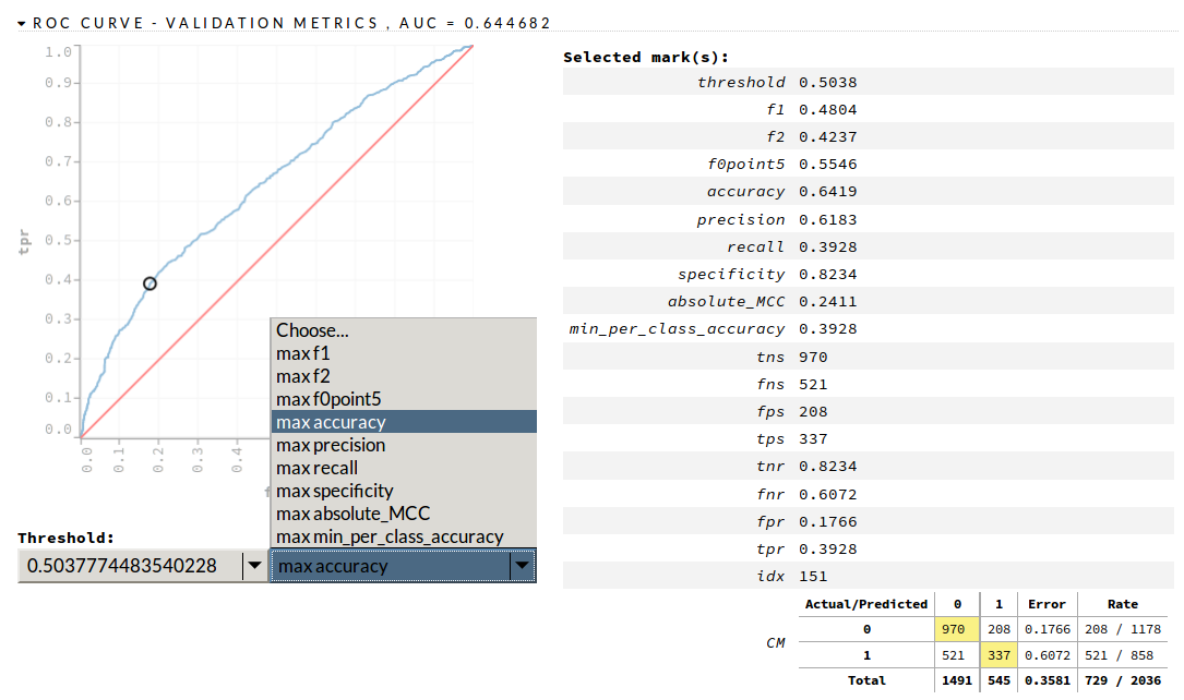
Figure 4-1. Example AUC plot in H2O’s Flow interface
You want a high AUC; you can see here it is 0.64. If it was 0.99 you would see the blue line almost touching the top-left corner. From the drop-down box I chose “max accuracy,” which represents one point along the line, to give the information on the right of the screenshot.
What about when FP and FN are of equal importance? Then you want to concentrate on accuracy. Accuracy is (TP + TN) / (TP + TN + FN + FP). That is, the total number correct over the total number of cases. Another way of saying that is 1 - error rate.
By default, H2O uses the F1-optimal threshold; we will instead use the threshold of maximum accuracy because, with the football predictions, the downside for guessing a win when it was a loss and for guessing a loss when it was a win are equal. When evaluating on the test data set, that threshold will be calculated as the average of the threshold that gave maximum accuracy on the train and validation data.
In Figure 4-2 the solid vertical lines show the threshold for maximum accuracy; the dotted line shows the average of the train and validation thresholds. Not perfect, but close enough.
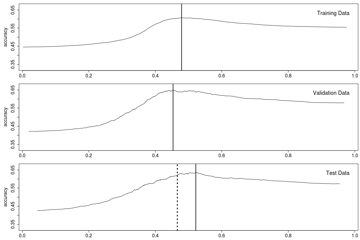
Figure 4-2. Binomial accuracy thresholds
The Essentials
All the machine learning algorithms have fields for what is being learned. In Python, the first three are given to train(), not when creating the estimator object:
- x
-
Which fields in
training_frameto learn from. The convention in this book is to store them in a variable also calledx.
- y
-
Which field in
training_frameshould be learned; in other words, which is the response variable. The convention in this book is to store it in a variable also calledy. (When doing unsupervised learning do not sety.) If doing regression this has to represent anumericfield, if doing binomial classification this has to represent a two-levelenum, and if doing multinomial classification this has to represent anenumwith three or more levels. - training_frame
-
The (handle to the H2O) data set to train from. The convention in this book is to call this
train. - ignore_const_cols
-
Defaults to true, meaning if all values in a column are the same value, then ignore that column. You usually only set it to false if you want to see it shown in reports, or they represent a 2D image you will want to plot.
In R, the first three arguments are always x, y, training_frame, in that order, and so you can skip naming them.2 That is, you can either do h2o.gbm(x, y, train) or h2o.gbm(x = x, y = y, training_frame = train). In Python it is the same: either m.train(x, y, train) or m.train(x=x, y=y, training_frame=train).
Typically, x and y are text: the names of fields. However, if your columns have no names, or there are a lot of columns, you can also use numeric indices, as we did with the MNIST data in the previous chapter. Either way, remember that x and y are column names or column indices, not the column data itself.
Caution
When using numeric column indices, in R they count from 1, in Python they count from 0, i.e., exactly what you’d expect in each language. Just be careful if sharing code with someone using a different language!
If you look on Flow, or ever use the REST API directly, you will see only column names are used, never numeric column indices. Also, rather than specifying the column names to use you specify which columns to ignore. So response_column on Flow is what we call y, and ignored_columns is the inverse of our x.
For instance, in Examples 4-1 and 4-2 we will try to learn the iris species from just the sepal width. Either of the first two ways is fine, but the third way, in each case, will give errors.
Example 4-1. Ways to give x and y (in R)
m1<-h2o.gbm(2,5,train)m2<-h2o.gbm("sepal_wid","class",train)m3<-h2o.gbm(train["sepal_wid"],train["class"],train)#BAD
Example 4-2. Ways to give x and y (in Python)
m=h2o.H2OGradientBoostingEstimator()m.train(1,4,train)m.train("sepal_wid","class",train)m.train(train["sepal_wid"],train["class"],train)#BAD
Effort
The first three items here tell their respective algorithms how much work to do:
- epochs
-
The amount of training cycles a deep learning algorithm should do.
- ntrees
-
The number of trees a tree algorithm should do.
- max_iterations
-
The amount of work a GLM algorithm should do (not applicable in cases when coefficients can be calculated directly).
The other couple of parameters allow you to set a random seed to get the exact same results again. Useful for demos, and book authors, but it is better to embrace stochastic diversity the way you would embrace a favorite aunt—without a second thought:
- seed
-
An integer to control random number generation, which allows you to get exactly the same model if you run the algorithm again. If using deep learning, you also need to set
reproducible. Perhaps ironically, my main use forseedis in grids (a way to tune model parameters, introduced properly in “Grid Search” in the next chapter) not to allow repeatability, but to allow me to run the same model with the same parameters and see what effect random variation has on the result. (When used for this purpose, you don’t need to setreproducible.) - reproducible
-
If true, then deep learning will run on a single thread. This takes away the random element, but of course means it will train more slowly. Set this if also setting a seed, don’t set it if not.
Warning
Setting a seed cannot guarantee you the same model results between different H2O versions. Bug fixes, new bugs, something as simple as a new feature, can be enough.
Scoring and Validation
H2O regularly scores how the model training is doing. If you give a validation_frame then it will score it on that, if you are using cross-validation, it will score against each fold, and if neither of those it will score against training_frame:
- validation_frame
-
The (handle to the H2O) data set to validate against. The convention in this book is to call this
valid. (In Python, this is given totrain(), not when creating the estimator.) - score_each_iteration
-
This defaults to false; if true it will do the scoring more frequently.
- score_tree_interval
-
The default of zero disables this. If you set it then the score is evaluated after this many trees.
Deep learning has a large number of additional scoring parameters, which are covered in “Parameters” in Chapter 8.
Early Stopping
As described in “Scoring and Validation”, H2O is regularly scoring your model against the validation, cross-validation, and/or training data. If you are using the Flow interface you can watch how the learning is going. Say you have a deep learning model, which you gave 1000 epochs, and you are regularly watching how it is doing. After 150 epochs you can see it has completely flattened out. You give it another 20 epochs to be sure, but after those it is clear it has learned all it is going to, and is now just wasting time. You yawn, and abort it.
That can get to a person’s sanity if you have to do it more than once or twice. Fortunately, H2O has some options to help. The first three are basically doing what you did manually earlier: watching your metric of choice, and when it has not improved for a certain number of scoring rounds, stop.
- stopping_metric
-
How to decide if the model is improving or not. “Supported Metrics” introduced the choices, though you can usually leave it as the default of AUTO (“logloss” for classification and “deviance” for regression).
- stopping_tolerance
-
Stop if it (your metric of choice) has not improved by at least this much. For example, 0.01 means you want a 1% improvement, or it should stop. Zero is also fine: it is saying to keep learning while there is any improvement, however small.
- stopping_rounds
-
The scoring history graphs for your models sometimes wobble around a bit. By setting this higher than 1 you make space for things to get worse before they get better. It works by comparing two moving averages; the earliest it can ever stop is after twice this number of scoring rounds. Choosing 1 means the model has to improve on every single scoring round. Set it to zero to not use early stopping at all.
How responsive your early stopping is depends not just on stopping_rounds and stopping_tolerance but also on how frequently scoring rounds happen. As an example, if the combination of your model complexity, training data size, and parameters you’ve set means that it only scores once a minute, and stopping_rounds is 5, then the earliest a model can ever stop training is after 10 minutes (twice the number in stopping_rounds). If using a grid (see “Grid Search”) this applies for each model that is made.
There are some other parameters that can stop a model early, though you will use them less often:
- max_runtime_secs
-
The maximum amount of time allowed for model training. The default of zero means no limit. This is cruder than using a stopping metric, but is more predictable: if you are making 50 models in a grid, and you set
max_runtime_secsto 30 seconds, then you know that (a) it will finish within 25 minutes and (b) each model will get the same amount of CPU resources, which may be the most fair comparison. (In Python, this is given totrain(), not when creating the estimator.) - classification_stop
-
When the classification error is below this, training will stop. Set it to –1 to not use this. This works independently of
stopping_metric. - regression_stop
-
When the MSE is below this, training will stop. Set it to –1 to not use this. This works independently of
stopping_metric. - max_active_predictors
-
Stops when there are more than this number of active predictors. The default of –1 means no limit.
- overwrite_with_best_model
-
True by default, which means the model that is returned will be the best model found during training. If false, then the final model (which may be inferior) will be the one that is returned. I’ve put it in this section, but this is also used even if not using early stopping.
H2O has early stopping on by default for deep learning, so explicitly set stopping_rounds to 0 if you don’t want it. My suggestion is to always use it for deep learning, if only because the overwrite_with_best_model feature means it can go back through the history and choose the best model, not whatever you ended up with at the end of training. For random forest and GBM, I recommend you either use early stopping or checkpoints, explained in a moment, or both.
The following example shows a random forest model that will keep adding trees unless one of three things has happened:
-
It uses 100 trees (
ntrees=100). -
It takes 60 seconds (
max_runtime_secs=60). -
The value for the misclassification metric has not improved by 2% over the last 3 scoring rounds.
This example uses the same Iris data set we saw back in the first chapter; in fact the first half is exactly the same as Example 1-1. But I’m now splitting off a validation frame, so my training data is reduced to 75% (e.g., 115 rows), and my test data is reduced to 10% (e.g., 16 rows), leaving me 15% for validation (e.g., 19 rows). (The split is random, so will be slightly different each time, unless you use seed.)
importh2oh2o.init()datasets="https://raw.githubusercontent.com/DarrenCook/h2o/bk/datasets/"data=h2o.import_file(datasets+"iris_wheader.csv")y="class"x=data.namesx.remove(y)train,valid,test=data.split_frame([0.75,0.15])fromh2o.estimators.random_forestimportH2ORandomForestEstimatorm=H2ORandomForestEstimator(ntrees=100,stopping_metric="misclassification",stopping_rounds=3,stopping_tolerance=0.02,#2%max_runtime_secs=60,model_id="RF:stop_test")m.train(x,y,train,validation_frame=valid)
In fact it stopped after using 8 trees, and 0.024 seconds of training!
Note
When used with cross-validation (explained in a moment) it will use your early stopping criteria on each cross-validation model. But from that it will work out the optimal number of trees/epochs and make the final model without using early stopping. (If model quality varies a lot from run to run, randomly, this can sometimes give strange results.)
Checkpoints
Imagine you spend 10 minutes training a neural net. Then you test it and find it has improved over the one you only trained for 5 minutes. So then you wonder how good it would be if you gave it 15 minutes. Altogether it takes you 30 minutes to discover those three things. H2O has this great feature, allowing you to train a model for 5 minutes then stop it and try it out. Then you can train it for another 5 minutes, giving you (approximately) the 10-minute model. And then another 5 minutes to give you the 15-minute model. The same three models, but in half the time.
There are two variables involved:
- model_id
-
A name for your model. If not given, a random one is chosen.
- checkpoint
-
The ID of a previous model (which must currently be on your H2O cluster) that you would like to use as a starting point.
Once you start any serious work with H2O, whether using checkpoints or not, I recommend you always set model_id, if only so you can find them in Flow, or find the saved model on disk. POJOs also get named based on the model ID. And for the same reasons, I recommend some convention. For example, “DL:200x200-100” could be a deep learning model with two hidden layers each with 200 neurons, and running for 100 epochs. “GBM:100-5” could be a GBM built with 100 trees, and a max depth of 5.
Tip
Don’t get carried away with structuring your model IDs: the more information you put in them, the less useful they get. If you find yourself wanting to put more than three parameters in a model ID, maybe it is time to step back and give them names instead. “DL:extra-deep,” “DL:big-and-slow,” etc. Or even “DL:Tom,” “DL:Dick,” and “DL:Harry.”
The way checkpoints work is you define a new model, with all the same parameters (usually: see the following comment), but give a higher value for epochs (deep learning) or ntrees (GBM, random forest), and then set checkpoint to the ID of the model to use as a starting point. If you give a lower or equal value for epochs/ntrees/max_iterations, then it will return immediately, as there is no new work to be done.
Example 4-3 shows how to build a model "DL:50x50-5" with 5 epochs, then use that as the starting point for a new model "DL:50x50-15", which we give another 10 epochs. When specifying epochs, or the number of trees, specify the total amount of training you want if you had started from scratch (epochs=15 here), not how many additional epochs or trees you want.
Example 4-3. Using checkpoints with deep learning (Python)
y="income"x=["age","gender"]m1=h2o.H2ODeepLearningEstimator(model_id="DL:50x50-5",hidden=[50,50],epochs=5)m1.train(x,y,train)m2=h2o.H2ODeepLearningEstimator(model_id="DL:50x50-15",hidden=[50,50],epochs=15,checkpoint="DL:50x50-5")m2.train(x,y,train)
If we look at m1.scoring_history()3 it looks like this:
 duration    epochs training_MSE
0.000 sec  0.000000     NaN
0.156 sec  0.471545     0.224481
0.205 sec  5.048780     0.036641
And m2.scoring_history() looks like this:
 duration    epochs training_MSE
0.000 sec  0.000000     NaN
0.156 sec  0.471545     0.224481
0.205 sec  5.048780     0.036641
0.261 sec  6.504065     0.096397
0.312 sec 15.455285     0.021673
The first three lines are identical! When checkpointing, the new model inherits all that information from the previous model.
One interesting aspect of checkpoints is that you can change more parameters than just how long to train, and thus create models that couldn’t be created without checkpoints. For instance, you can use a certain dropout ratio for the first 50 epochs of a deep learning model, then switch to a different dropout ratio for the next 50.
Tip
When I started using H2O, I thought checkpoints were the bees knees, and used them a lot. But now (at least when using deep learning and I have a validation data set) I prefer to use “Early Stopping” to decide how much to train a model, and instead only use checkpoints for when I feel early stopping has stopped too soon. Or the scenario described in “Model Files”, where I want to shut down a cluster for the weekend but a model is still learning. (You can export the latest snapshot of a model from Flow, while it is learning.)
Cross-Validation (aka k-folds)
The basic idea behind cross-validation is you chop up your training set into k blocks, then use one of those k blocks as a validation data set, and use the rest for training. Repeat this k times, with a different part of the training set being the validation set each time. The error of the final model is estimated as the average error of the k models and it should therefore be more reliable. The final model that is returned is built again, with all the data, and no validation. The cost of this more reliable estimate of model quality is that it takes more time. Figure 4-3 shows the process for three random folds. m is the final model that is returned.
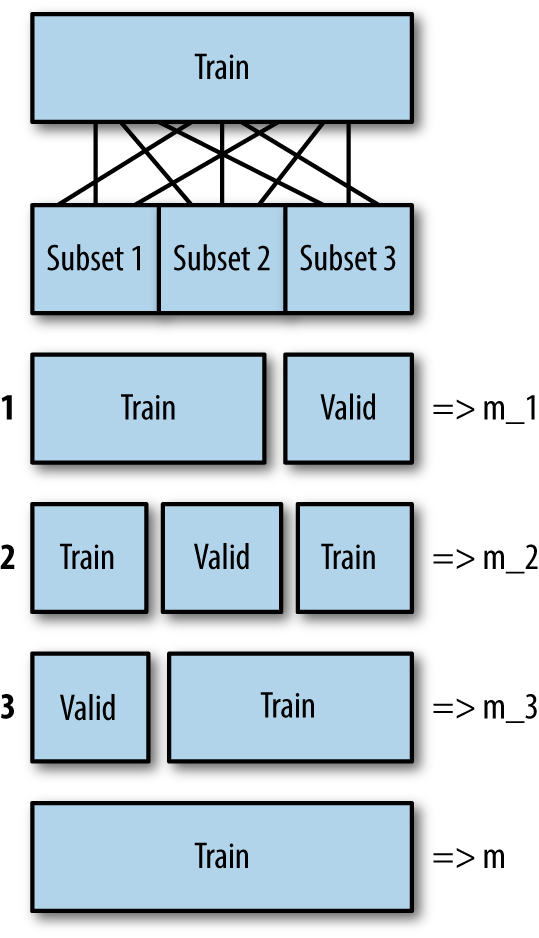
Figure 4-3. The cross-validation process for k=3
In this book I use cross-validation for the building energy data set, but a validation data set for MNIST (as I have enough data) and the football statistics (as I have enough data and it is a time series).
- nfolds
-
Number of folds. The higher this is the longer training takes, but the more accurate the error estimate, meaning an overfitted model is harder to get past us. However, there are diminishing returns. 5 and 10 are common choices for
nfolds.
The next two parameters control how the data is split up. Generally there is no need to touch these. However, if doing a classification, and the classes are not balanced, consider fold_assignment="Stratified".
- fold_assignment
-
How to split up the training data. The choices are “Random,” “Modulo,” and “Stratified,” with the default being “AUTO” (which always means Random, at the moment).
Randomis what you’d expect, and each fold might end up a slightly different size. Ifnfoldsis 3,Modulomeans rows 1, 4, 7, … go into fold 1, rows 2, 5, 8, … go into fold 2, and rows 3, 6, 9, … go into fold 3.Stratifiedtries to get the same amount of each target class into each fold; this is a good thing but splitting the data might take more time. - fold_column
-
Allows you complete control. If
nfoldsis 3, then this column should contain the values 1, 2, and 3 to say which fold you want each row in. (In Python, this is given totrain(), not when creating the estimator.)
The final two parameters are boolean, to control what information is returned:
- keep_cross_validation_fold_assignment
-
If set to true then you can find out which rows were in which folds.
- keep_cross_validation_predictions
-
If set to true then the predictions of the test step for each fold are kept.
Tip
To use models with h2o.stack(), a technique described in “Ensembles” in Chapter 10, you must use cross-validation, and must set fold_assignment = "Modulo" and keep_cross_validation_predictions = TRUE. If you think that is something you might want to do, it can be worth choosing those options on all your models.
Data Weighting
If you have 100 rows of training data, all 100 are considered equally important. H2O provides a few ways to describe that certain rows are more important, without you having to resort to taking a copy of your training data and actually duplicating the rows. All of them can be used with each of the learning algorithms. The first three only apply when doing a classification:
- balance_classes
-
If false, all data is used evenly. If set to true, then training data class counts (for your response variable) will be used to over/under-sample. For example, assume you are predicting favorite color, and in your 100 training rows 40 people chose red, 30 chose blue, 15 chose black, 10 chose white, 4 chose orange, and only 1 chose green. With
balance_classeson, each of the blue rows will be made 1.33 times more important than each of the red rows, the black rows will be 2.67 times more important than each of the red rows, and so on, down to the single green row, which will be 40 times more important. - class_sampling_factors
-
Allows explicit control when using
balance_classes. The default is to balance so that all classes are equally balanced. You should only set this if that equal balancing is not desired. The entries should be in sort order. For example, if you want the same ratio of colors as just shown but also want to limit the maximum weight of any one color to 5.0, you would give:[2.67, 1.33, 5.0, 5.0, 1.0, 4.0](i.e., black, blue, green, orange, red, white is their alphabetic sorted order). Also see the following example, where we happen to know that the training data is not representative. - max_after_balance_size
-
When using
balance_classes, this allows you to set the maximum relative size of the training data after balancing. Currently this defaults to 5.0, and you are unlikely to need to change it.
Note
With h2o.deeplearning() when using balance_classes, it is recommended to also set shuffle_training_data to TRUE. (shuffle_training_data is only a parameter for h2o.deeplearning()).
The other two are more general:
- weights_column
-
The name of a column that says how to weight each row. You can think of this as being how many times to repeat each row when training, so the default is like an invisible column with 1.0 for every row. Fractional values are allowed. Cannot be used when
balance_classesis set. (In Python, this is given totrain(), not when creating the estimator.) - offset_column
-
The name of a column that gives a per-row bias. You can think of the default as being an invisible column with 0.0 for every row. It is like copying and modifying your response variable column by this much, for each row. (In Python, this is given to
train(), not when creating the estimator.)
Here is a full example of using each of the choices for balancing classes:
library(h2o)h2o.init(nthreads=-1)datasets<-"https://raw.githubusercontent.com/DarrenCook/h2o/bk/datasets/"data<-h2o.importFile(paste0(datasets,"iris_wheader.csv"))data<-data[1:120,]#Remove 60% of virginicasummary(data$class)#50/50/20parts<-h2o.splitFrame(data,0.8)train<-parts[[1]]test<-parts[[2]]summary(train$class)#41/41/14summary(test$class)#9/9/6m1<-h2o.randomForest(1:4,5,train,model_id="RF_defaults")h2o.confusionMatrix(m1)m2<-h2o.randomForest(1:4,5,train,model_id="RF_balanced",balance_classes=TRUE)h2o.confusionMatrix(m2)m3<-h2o.randomForest(1:4,5,train,model_id="RF_class_sampling",balance_classes=TRUE,class_sampling_factors=c(1,1,2.5))h2o.confusionMatrix(m3)
The first four lines are hopefully familiar by now: start H2O, and load the iris data. I then throw away the last 30 samples (which are all virginica), by keeping just rows 1 to 120. I now have an unbalanced data set: 50 setosa, 50 versicolor, 20 virginica. I chose the seed deliberately when splitting the data, such that my training data has 41 setosa, 41 versicolor, 14 virginica. That is, virginica is 14.58% of the training data and 25% in the test data, compared to 16.67% overall.
I then train three random forest models. m1 is all defaults, and its confusion matrix looks like this:
           setosa versicolor virginica  Error     Rate
setosa         41          0         0 0.0000 = 0 / 41
versicolor      0         39         2 0.0488 = 2 / 41
virginica       0          1        13 0.0714 = 1 / 14
Totals         41         40        15 0.0312 = 3 / 96
Nothing to see here: it uses the data as it finds it.
Now here is the same output for m2, which switches on balance_classes. You can see it has over-sampled the virginica class to get them as balanced as possible (the rightmost column says 41,41,40 instead of 41,41,14 as in the previous output):
           setosa versicolor virginica  Error      Rate
setosa         41          0         0 0.0000 =  0 / 41
versicolor      0         41         0 0.0000 =  0 / 41
virginica       0          2        38 0.0500 =  2 / 40
Totals         41         43        38 0.0164 = 2 / 122
In m3 we still switch on balance_classes, but also tell it the truth of the situation. That is, that the actual data is 16.67% virginica, not the 14.58% it sees in the train data. The confusion matrix for m3 shows that it turned the 14 virginica samples into 37 samples instead of 40 samples:
           setosa versicolor virginica  Error      Rate
setosa         41          0         0 0.0000 =  0 / 41
versicolor      0         41         0 0.0000 =  0 / 41
virginica       0          2        35 0.0541 =  2 / 37
Totals         41         43        35 0.0168 =  2 /119
How did I know to write c(1, 1, 2.5), and not c(2.5, 1, 1) or c(1, 2.5, 1)? You can find out the correct order with h2o.levels(train$class) which tells me:
[1] "setosa" "versicolor" "virginica"
Sampling, Generalizing
The common theme among the parameters in this section is that they try to improve your model’s ability to generalize, and they do this by hiding some of the data. Generalization is a good thing; it means your model can make a good guess when it sees some combination of inputs that it has never encountered before. But, hiding some of the data?! Surely the machine learning is hard enough, and the more data the better?
Imagine you are teaching trigonometry, and you teach the students about sine and tangent, but not about cosine. You then give them a test, and kick out of the class anyone who obviously hasn’t worked out the existence of cosine for themselves. This is a good way to make parents angry and get yourself sacked. But it is also a great way to discover who are the budding mathematical geniuses and who merely pay attention in class but don’t really get it.
Leaving that metaphor behind, it is important to realize that if you hide information, you often need to spend more time learning. With the tree algorithms, you need to give them more trees, and with deep learning you need to give it more epochs. So it will take longer to train, but (hopefully) give a more resilient model.
I only show the parameters for the tree algorithms here. Those for deep learning are in “Deep Learning Regularization” and those for GLM are in “GLM Parameters”. In all cases they are hard to select even with good knowledge of the data, so they are good candidates for a grid search.
For the tree algorithms the parameters are about two things:
-
Use all columns?
-
Use all training rows?
- mtries
-
This is how many variables to randomly choose as candidates at each split, in a random forest. The default is –1, which means
 (rounded down, minimum of 1) for classification, or P/3 (rounded down, minimum of 1) for regression (where P is the number of columns).
 - col_sample_rate
-
This is the percentage of columns (from 0.0 to 1.0) to sample from, with GBM. The default is 1. If you multiply
col_sample_rateby the number of columns intrain, you get the equivalent ofmtries. - col_sample_rate_change_per_level
-
Relative change of the column sampling rate for every level in each tree. The default is 1.0. If less than 1, then it will have fewer columns to choose from as it gets deeper in the tree. If greater than 1 (maximum 2.0), then it will have more columns to choose from. You might want to experiment with this in a grid, but normally you can just leave it as the default.
- col_sample_rate_per_tree
-
This can be from 0.0 to 1.0. It is at the tree level, rather than at the split level as with
mtriesandcol_sample_rate. The default is 1.0. - sample_rate
-
The default for GBM is 1.0, which means train each tree on all the training data. 0.5 would mean only use half the data. The default for random forest is 0.632.
- sample_rate_per_class
-
Like
sample_ratebut you give the value for each class. See the description ofclass_sampling_factorsunder “Data Weighting”. - max_abs_leafnode_pred
-
Maximum absolute value of a leaf node prediction. This is the maximum a leaf node can contribute, so it is a regularization parameter. It defaults to a very large number, but if set lower it stops any one node from dominating the prediction. Generally it can be left as the default, but it might be worth experimenting with in a grid.
Regression
Regression is trying to predict a (continuous) number (as different from a classification), and there are a few parameters specifically to control regression.
These first few only apply to deep learning and GBM:
- distribution
-
Choose the probability distribution of the response variable; the choices are listed in a moment.4 The default is “AUTO,” which is always “gaussian” for a regression. (For binomial classification, distribution is always “bernoulli,” and for multinomial classification it is always “multinomial.”)
- quantile_alpha
-
Used when distribution is “quantile.”
- tweedie_power
-
Used when distribution is “tweedie.” From 1.0 to 2.0, defaulting to 1.5. Note that 1.0 is equivalent to “poisson,” while 2.0 is equivalent to “gamma.”
- loss
-
Certain distributions (gaussian, laplace, huber) allow you to choose a loss function. The default choices for those three being: “Quadratic,” “Absolute,” “Huber.” The final possible value is “CrossEntropy,” which is for classification. Give the default of “Automatic” unless you have a good reason not to. You cannot define your own loss function.
These ones are for GLM:
- family
-
As
distributionbut for GLMs. The choices are listed next, but note that only gaussian, poisson, gamma, and tweedie are available (i.e., not huber, laplace, or quantile.) - tweedie_link_power
-
Used when distribution is “tweedie.” Default is 1.
- tweedie_variance_power
-
Used when distribution is “tweedie.” Default is 0.
Output Control
In this final group are a few parameters that control what information is reported back to the client. With some it is about controlling verbosity; with others it is about avoiding extra machine load if you do not need the extra information:
- max_hit_ratio_k
-
The maximum number of predictions to report in hit ratios (only applies to multinomial classification). Use 0 to disable (meaning it will make predictions for all classes).
- max_confusion_matrix_size
-
Maximum number of classes to use when printing confusion matrices in the logs.
- export_weights_and_biases
-
Set this to true to request to save a deep learning model’s weights and biases. They are available afterwards with
h2o.weights()andh2o.biases()(or member functions of those names, in Python). - variable_importances
-
The other learning algorithms always tells you relative importance of your input variables, but it can slow down deep learning; therefore it is off by default. Set this to true to have them calculated and returned.5
- diagnostics
-
Enable diagnostics for hidden layers.
- compute_p_values
-
Request p-values computation for your linear model. Only available when using the IRLSM solver and no regularization. (The latter limits its usefulness more than the former.)
Summary
That was a lot of parameters! But, along the way, we also got a look at some key concepts in machine learning and H2O: cross-validation and validation data sets, early stopping, scoring metrics, checkpoints, dealing with unbalanced data, random sampling to improve model generalization, and probability distributions.
The next chapter starts our four chapter tour of the supervised machine learning algorithms. And, because it is the first of the four, it will also introduce some techniques that apply to all of them, grid search in particular.
1 See http://data.library.virginia.edu/is-r-squared-useless/ for a good explanation of why.
2 If your coding standards and/or coworkers and/or boss allow it.
3 m1.scoring_history()[['duration','epochs','training_MSE']] was used here; there are lots of other columns telling you how training progressed, but we don’t want to see them in this example.
4 If you have questions about exactly what a distribution does, the Java source is authoritative.
5 The implementation is based on Gedeon, and the code for computeVariableImportances() is in http://bit.ly/2f8ewED. It uses the first two layers, so could be inaccurate for very deep networks, but it is only an estimate anyway.
Get Practical Machine Learning with H2O now with the O’Reilly learning platform.
O’Reilly members experience books, live events, courses curated by job role, and more from O’Reilly and nearly 200 top publishers.

