VLSI Digital Signal Processing Systems: Design and Implementation

12.6    DERIVATION OF SCALED-NORMALIZED LATTICE FILTER

By applying the slow-down and retiming/pipelining (SRP) transformation (see Section 11.7) with M = 2 to a 3rd-order normalized lattice filter, we obtain the filter structure in Fig. 12.17. In Fig. 12.17, each delay element is represented by x_i, for i = 1 to 8, and is denoted by c_i, for i = 0 to 3. From (12.74), each x_i(n), for i = 3 to 8, has unit power. In terms of the state covariance matrix, K_ii = 1, for i = 3 to 8, where K_ii is the i-th diagonal element of K. Then, to scale the filter, we only need to compute the powers of x₁(n) and x₂(n), which can be computed from (11.25). In the case of the normalized lattice filter, K₁₁ and K₂₂ can be computed more efficiently using the orthonormality of the Schur polynomials. From Fig 12.17, the polynomial at the state x₁ is given by:

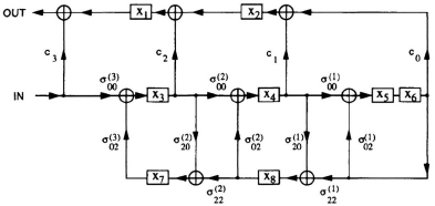
Fig. 12.17    A 3rd-order normalized lattice filter after upsampling and retiming with M = 2.

Therefore, using the orthonormality of the Schur polynomials,

By the same way,

In general, for the summing node on the top line of module i, the power is . To have ...