The first thing you should do in tuning a web site is to monitor that site so you can see patterns and trends. From this you’ll know whether you’re helping or not. And as we will see later, the same programs we write for monitoring can also be used for load testing.
In this chapter, we first define some parameters of performance. Then we show how to monitor them with free software from http://patrick.net/, without installing anything on production machines.
There are four classic parameters describing the performance of any computer system: latency, throughput, utilization, and efficiency. Tuning a system for performance can be defined as minimizing latency and maximizing the other three parameters. Though the definition is straightforward, the task of tuning itself is not, because the parameters can be traded off against one another and will vary with the time of day, the sort of content served, and many other circumstances. In addition, some performance parameters are more important to an organization’s goals than others.
Latency is the time between making a request and beginning to see a result. Some define latency as the time between making a request and the completion of the response, but this definition does not clearly distinguish the psychologically significant time spent waiting, not knowing whether a request has been accepted or understood. You will also see latency defined as the inverse of throughput, but this is not useful because latency would then give you the same information as throughput. Latency is measured in units of time, such as seconds.
Throughput is the number of items processed per unit time, such as bits transmitted per second, HTTP operations per day, or millions of instructions per second (MIPS). It is conventional to use the term “bandwidth” when referring to throughput in bits per second. Throughput is found by adding up the number of items and dividing by the sample interval. This calculation may produce correct but misleading results because it ignores variations in processing speed within the sample interval.
The following examples help clarify the difference between latency and throughput:
An overnight (24-hour) shipment of 1000 different CDs holding 500 megabytes each has terrific throughput but lousy latency. The throughput is (500 × 220 × 8 × 1000) bits/(24 × 60 × 60) seconds = about 49 million bits/second, which is better than a T3’s 45 million bits/second. The difference is the overnight shipment bits are delayed for a day and then arrive all at once, but T3 bits begin to arrive immediately, so the T3 has much better latency, even though both methods have approximately the same throughput when considered over the interval of a day. We say that the overnight shipment is bursty traffic. This example was adapted from Computer Networks by Andrew S. Tanenbaum (Prentice Hall, 1996).
Trucks have great throughput because you can carry so much on them, but they are slow to start and stop. Motorcycles have low throughput because you can’t carry much on them, but they start and stop more quickly and can weave through traffic so they have better latency.
Supermarkets would like to achieve maximum throughput per checkout clerk because they can then get by with fewer clerks. One way for them to do this is to increase your latency — that is, to make you wait in line, at least up to the limit of your tolerance. In his book Configuration and Capacity Planning for Solaris Servers (Prentice Hall), Brian Wong phrased this dilemma well by saying that throughput is a measure of organizational productivity while latency is a measure of individual productivity. The supermarket may not want to waste your individual time, but it is even more interested in maximizing its own organizational productivity.
One woman has a throughput of one baby per nine months, barring twins, triplets, etc. Nine women may be able to bear nine babies in nine months, giving the group a throughput of one baby per month, even though the latency cannot be decreased (i.e., even nine women cannot produce one baby in one month). This mildly offensive but unforgettable example is from The Mythical Man-Month by Frederick P. Brooks (Addison Wesley).
Although high throughput systems often have low latency, there is no causal link. You’ve just seen how an overnight shipment can have high throughput with high latency. Large disks tend to have better throughput but worse latency; the disk is physically bigger, so the arm has to seek longer to get to any particular place. The latency of packet network connections also tends to increase with throughput. As you approach your maximum throughput, there are simply more or larger packets to put on the wire, so a packet will have to wait longer for an opening, increasing latency. This is especially true for Ethernet, which allows packets to collide and simply retransmits them if there is a collision, hoping that it retransmitted them into an open slot. It seems obvious that increasing throughput capacity will decrease latency for packet switched networks. However, while latency due to traffic congestion can be reduced, increasing bandwidth will not help in cases in which the latency is imposed by routers or sheer physical distance.
Finally, you can also have low throughput with low latency: a 14.4 kbps modem may get the first of your bits back to you reasonably quickly, but its relatively low throughput means it will still take a tediously long time to get a large graphic to you. With respect to the Internet, the point to remember is that latency can be more significant than throughput. For small HTML files, say under 2K, more of a 28.8 kbps modem user’s time is spent between the request and the beginning of a response than waiting for the file to complete its arrival.
A graph of latency versus load is very different from a graph of throughput versus load. Latency will go up exponentially, making a characteristic “backwards L"- shaped graph. Throughput will go up linearly at first, then level out to become nearly flat. Simply by looking at a graph of load test results, you can immediately have a good idea whether it is a latency or throughput graph.
Each step on the network from client to server and back contributes to the latency of an HTTP operation. It is difficult to figure out where in the network most of the latency originates, but there are two commonly available Unix tools that can help. (Note that we’re considering network latency here, not application latency, which is the time the applications running on the server itself take to begin to put a result back out on the network.)
If your web server is accessed over the Internet, then much of your latency is probably due to the store-and-forward nature of routers. Each router must accept an incoming packet into a buffer, look at the header information, and make a decision about where to send the packet next. Even once the decision is made, the router will often have to wait for an open slot to send the packet. The latency of your packets will therefore depend strongly on the number of router hops between the web server and the user. Routers themselves will have connections to each other that vary in latency and throughput.
The odd but essential characteristic about the Internet is the path between two end-points can change automatically to accommodate network trouble, so your latency may vary from packet to packet. Packets can even arrive out of order. You can see the current path your packets are taking and the time between router hops by using the traceroute utility that comes with most versions of Unix. (See the traceroute manpage for more information.) A number of kind souls have made traceroute available from their web servers back to the requesting IP address, so you can look at path and performance to you from another point on the Internet, rather than from you to that point. One page of links to traceroute servers is at http://www.slac.stanford.edu/comp/net/wan-mon/traceroute-srv.html. Also see http://www.internetweather.com/ for continuous measurements of ISP latency as measured from one point on the Internet.
Note that by default traceroute does a reverse DNS lookup on all intermediate IPs so you can see their names, but this delays the display of results. You can skip the DNS lookup with the -n option and you can do fewer measurements per router (the default is three) with the -q option. Here’s an example of traceroute usage:
% traceroute -q 2 www.umich.edu
traceroute to www.umich.edu (141.211.144.53), 30 hops max, 40 byte packets
1 router.cableco-op.com (206.24.110.65) 22.779 ms 139.675 ms
2 mv103.mediacity.com (206.24.105.8) 18.714 ms 145.161 ms
3 grfge000.mediacity.com (206.24.105.55) 23.789 ms 141.473 ms
4 bordercore2-hssi0-0.SanFrancisco.mci.net (166.48.15.249) 29.091 ms 39.856 ms
5 bordercore2.WillowSprings.mci.net (166.48.22.1) 63.16 ms 62.75 ms
6 merit.WillowSprings.mci.net (166.48.23.254) 82.212 ms 76.774 ms
7 f-umbin.c-ccb2.umnet.umich.edu (198.108.3.5) 80.474 ms 76.875 ms
8 www.umich.edu (141.211.144.53) 81.611 ms *
If you are not concerned with intermediate times and want only to know the current time it takes to get a packet from your machine to another machine on the Internet (or on an intranet) and back to you, you can use the Unix ping utility. ping sends Internet Control Message Protocol (ICMP) packets to the named host and returns the latency between you and the named host as milliseconds. A latency of 25 milliseconds is pretty good, while 250 milliseconds is not good. See the ping manpage for more information. Here’s an example of ping usage:
% ping www.umich.edu
PING www.umich.edu (141.211.144.53): 56 data bytes
64 bytes from 141.211.144.53: icmp_seq=0 ttl=248 time=112.2 ms
64 bytes from 141.211.144.53: icmp_seq=1 ttl=248 time=83.9 ms
64 bytes from 141.211.144.53: icmp_seq=2 ttl=248 time=82.2 ms
64 bytes from 141.211.144.53: icmp_seq=3 ttl=248 time=80.6 ms
64 bytes from 141.211.144.53: icmp_seq=4 ttl=248 time=87.2 ms
64 bytes from 141.211.144.53: icmp_seq=5 ttl=248 time=81.0 ms

--- www.umich.edu ping statistics ---

6 packets transmitted, 6 packets received, 0% packet loss
round-trip min/avg/max = 80.6/87.8/112.2 msWhen ping measures the latency between you and some remote machine, it sends ICMP messages, which routers handle differently than the TCP segments used to carry HTTP. ICMP packets get lower priority. Routers are sometimes configured to ignore ICMP packets entirely. Furthermore, by default, ping sends only a very small amount of information, 56 data bytes, although some versions of ping let you send packets of arbitrary size. For these reasons, ping is not necessarily accurate in measuring HTTP latency to the remote machine, but it is a good first approximation. Using telnet and the Unix talk program will give you a manual feel for the latency of a connection.
The simplest ways to measure web latency
and throughput are to clear your browser’s cache and
time how long it takes to get a particular page from your server,
have a friend get a page from your server from another point on the
Internet, or log in to a remote machine and run: time lynx -source http://patrick.net/>/dev/null. This method is
sometimes referred to as the stopwatch method
of web performance monitoring.
Another way to get an idea of network throughput is to use FTP to transfer files to and from a remote system. FTP is like HTTP in that it is carried over TCP. There are some hazards to this approach, but if you are careful, your results should reflect your network conditions.
First, do not put too much stock in the numbers the FTP program reports to you. While the first significant digit or two will probably be correct, the FTP program internally makes some approximations, so the number reported is only approximately accurate.
More importantly, what you do with FTP will determine exactly which part of the system is the bottleneck. To put it another way, what you do with FTP will determine what you’re measuring. To insure that you are measuring the throughput of the network and not of the disk of the local or remote system, you want to eliminate any requirements for disk access that could be caused by the FTP transfer. For this reason, you should not FTP a collection of small files in your test; each file creation requires a disk access.
Similarly, you need to limit the size of the file you transfer because a huge file will not fit in the filesystem cache of either the transmitting or receiving machine, again resulting in disk access. To make sure the file is in the cache of the transmitting machine when you start the FTP, you should do the FTP at least twice, throwing away the results from the first iteration. Also, do not write the file on the disk of the receiving machine. You can do this with some versions of FTP by directing the result to /dev/null. Altogether, we have something like this:
ftp> get bigfile /dev/null
Try using the FTP hash
command to get an interactive feel for latency and throughput. The
hash command prints hash marks
(#) after the transfer of a block of data. The
size of the block represented by the hash mark varies with the FTP
implementation, but FTP will tell you the size when you turn on
hashing:
ftp> hash
Hash mark printing on (1024 bytes/hash mark).
ftp> get ers.27may
200 PORT command successful.
150 Opening BINARY mode data connection for ers.27may (362805 bytes).
#######################################################################################
226 Transfer complete.
362805 bytes received in 15 secs (24 Kbytes/sec)
ftp> bye
221 Goodbye.
You can use Perl or the Expect scripting language to automatically run an FTP test at regular intervals. Other scripting languages have a difficult time controlling the terminal of a spawned process; if you start FTP from within a shell script, for example, execution of the script halts until FTP returns, so you cannot continue the FTP session. Expect is designed to deal with this exact problem. Expect is well documented in Exploring Expect, by Don Libes (O’Reilly Media). The autoexpect program can be used to automatically record your test.
You can of course also retrieve content via HTTP from your server to test network performance, but this does not clearly distinguish network performance from server performance.
Here are a few more network testing tools:
- ttcp
ttcp is an old C program, circa 1985, for testing TCP connection speed. It makes a connection on port 2000 and transfers zeroed buffers or data copied from STDIN. It is available from ftp://ftp.arl.mil/pub/ttcp/ and distributed with some Unix systems. Try
which ttcpandman ttcpon your system to see if the binary and documentation are already there.- Nettest
A more recent tool, circa 1992, is Nettest, available at ftp://ftp.sgi.com/sgi/src/nettest/. nettest was used to generate some performance statistics for vBNS, the very high-performance backbone network service (see http://www.vbns.net/).
- bing
bing attempts to measure bandwidth between two points on the Internet. See http://web.cnam.fr/reseau/bing.html.
- chargen
The chargen service, defined in RFC 864 and implemented by most versions of Unix, simply sends back nonsense characters to the user at the maximum possible rate. This can be used along with some measuring mechanism to determine what that maximum rate is. The TCP form of the service sends a continuous stream, while the UDP form sends a packet of random size for each packet received. Both run on well-known port 19. chargen does not give reliable readings because it cannot distinguish between packets that were dropped on the sending machine from packets dropped at the receiving machine due to buffer overflows.
- NetSpec
NetSpec simplifies network testing by allowing users to control processes across multiple hosts using a set of daemons. It can be found at http://www.tisl.ukans.edu/Projects/AAI/products/netspec.old/.
Utilization is simply the fraction of the capacity of a component that you are actually using. You might think that you want all your components at close to 100 percent utilization in order to get the most bang for your buck, but this is not necessarily how things work. Remember that for disk drives and Ethernet, latency suffers greatly at high utilization. A rule of thumb is many components can run at their best performance up to about 70 percent utilization. The perfmeter tool that comes with many versions of Unix is a good graphical way to monitor the utilization of your system.
Efficiency is usually defined as throughput divided by utilization. When comparing two components, if one has a higher throughput at the same level of utilization, it is regarded as more efficient. If both have the same throughput but one has a lower level of utilization, that one is regarded as more efficient. While useful as a basis for comparing components, this definition is otherwise irrelevant, because it is only a division of two other parameters of performance.
A more useful measure of efficiency is performance per unit cost. This is usually called cost efficiency. Performance tuning is the art of increasing cost efficiency: getting more bang for your buck. In fact, the Internet itself owes its popularity to the fact that it is much more cost-efficient than previously existing alternatives for transferring small amounts of information. Email is vastly more cost-efficient than a letter. Both send about the same amount of information, but email has near-zero latency and near-zero incremental cost; it doesn’t cost you any more to send two emails rather than one.
Web sites providing product information have lower latency and are cheaper than printed brochures. As the throughput of the Internet increases faster than its cost, entire portions of the economy will be replaced with more cost-efficient alternatives, especially in the business-to-business market, which has little sentimentality for old ways. First, relatively static information such as business paperwork, magazines, books, CDs, and videos will be virtualized. Second, the Internet will become a real-time communications medium.
The cost efficiency of the Internet for real-time communications threatens not only the obvious target of telephone carriers, but also the automobile and airline industries. That is, telecommuting threatens physical commuting. Most of the workforce simply moves bits around, either with computers, on the phone, or in face-to-face conversations (which are, in essence, gigabit-per-second, low-latency video connections). It is only these face-to-face conversations that currently require workers to buy cars for the commute to work. Cars are breathtakingly inefficient, and telecommuting represents an opportunity to save money. Look at the number of cars on an urban highway during rush hour. It’s a slow river of metal, fantastically expensive in terms of car purchase, gasoline, driver time, highway construction, insurance, and fatalities. Then consider that most of those cars spend most of the day sitting in a parking lot. Just think of the lost interest on that idle capital. And consider the cost of the parking lot itself, and the office.
As data transmission costs continue to accelerate their fall, car costs cannot fall at the same pace. Gigabit connections between work and home will inevitably be far cheaper than the daily commute, for both the worker and employer. And at gigabit bandwidth, it will feel like you’re really there.
You can easily measure web performance yourself by writing scripts that time the retrieval of HTML from a web server — that is, the latency. If you have the text browser Lynx from the University of Kansas, here’s a simple way to get an idea of the time to get an answer from any server on the Internet:
% time lynx -source http://patrick.net/
0.05user 0.02system 0:00.74elapsed 9%CPU
(On some systems the time command has been replaced with timex). Of course, the startup time for Lynx is included in this, but if you run it twice and throw away the first result, your second result will be fairly accurate and consistent because the Lynx executable won’t have to be loaded from disk. Remember that network and server time is included as well. In fact, this includes all the time that is not system or user time: .67 seconds in the example above, which used a cable modem connection to a fast server. So even in the case of very good network connectivity, the Internet can still take most of the time. You can also get basic latency measurements with the free Perl tool webget in place of Lynx, or the simple GET program installed with the LWP Perl library.
A great thing about Lynx is that it is runnable via a Telnet session, so if you want to see how the performance or your site looks from elsewhere on the Internet, and you have an account somewhere else on the Internet, you can log in to the remote machine and run the time lynx command given earlier. The time given will be the time from the remote point of view. If you’d like to monitor the performance of a web server rather than just measure it once, the following trivial shell script will do just that. Note that we throw out the page we get by redirecting standard output to /dev/null, because we care only about how long it took. The time measurement will come out on standard error.
#!/bin/bash
while true
do
  time lynx -source http://patrick.net/ > /dev/null
  sleep 600
done
If you call the above script mon, then you can capture the results from standard error (file descriptor 2) to a file called log like this in bash:
$ mon 2>logShell scripting is about the least efficient form of programming because a new executable must be forked for almost every line in the script. Here is a tiny C program, modified from the example client in Chapter 11, which prints out the time it takes to retrieve the home page from a web site. It is much more accurate and efficient at run-time, but also much more complex to write. You can download it from http://patrick.net/software/latency.c.
#include <stdio.h>
#include <errno.h>
#include <netdb.h>
#include <netinet/in.h>
#include <sys/socket.h>
#include <sys/time.h>

#define PORT 80
#define BUFSIZE 4000

int main(int argc, char *argv[]) {
 int sockfd, count;
 char *request = "GET / HTTP/1.0\n\n";
 char reply[BUFSIZE];
 struct hostent *he;
 struct sockaddr_in target;
 struct timeval *tvs; /* start time */
 struct timeval *tvf; /* finish time */
 struct timezone *tz;

 if ((he=gethostbyname(argv[1])) == NULL) {
        herror("gethostbyname");
        exit(1);
 }

 if ((sockfd = socket(AF_INET, SOCK_STREAM, 0)) == -1) {
        perror("socket");
        exit(1);
 }

 target.sin_family = AF_INET;
 target.sin_port = htons(PORT);
 target.sin_addr = *((struct in_addr *)he->h_addr);
 bzero(&(target.sin_zero), 8);

 if (connect(sockfd, (struct sockaddr *)&target,
        sizeof(struct sockaddr)) == -1) {
        perror("connect");
        exit(1);
 }

 tvs = (struct timeval *) malloc(sizeof(struct timeval));
 tvf = (struct timeval *) malloc(sizeof(struct timeval));
 tz = (struct timezone *) malloc(sizeof(struct timezone));

 gettimeofday(tvs, tz);
 send(sockfd, request, strlen(request), 0);
 if ((count = recv(sockfd, reply, BUFSIZE, 0)) == -1) {
        perror("recv");
        exit(1);
 }
 gettimeofday(tvf, tz);

 printf("%d bytes received in %d microseconds\n", count,
        (tvf->tv_sec - tvs->tv_sec) * 1000000 +
        (tvf->tv_usec - tvs->tv_usec));
        close(sockfd);
        return 0;
}
Compile it like this:
% gcc -o latency latency.cAnd run it like this:
% latency patrick.netHere is sample output:
2609 bytes received in 6247 microseconds
While the C program does something we want, it is a bit too low-level to be conveniently maintained or updated. Here is a similar program in Perl, which is more efficient than shell scripting, but less efficient than C. We use the LWP::UserAgent library because it is easier than doing direct socket manipulation. We need to use the Time::HiRes library because timings are to whole second resolution by default in Perl.
#!/usr/local/bin/perl -w
use LWP::UserAgent;
use Time::HiRes 'time','sleep';

$ua = LWP::UserAgent->new;
$request = new HTTP::Request('GET', "http://$ARGV[0]/");
$start = time(  );
$response = $ua->request($request);
$end = time(  );
$latency = $end - $start;

print length($response->as_string( )), " bytes received in $latency seconds\n";We can easily expand on the earlier Perl example shown previously to create a useful monitoring system. This section shows how I set up an automated system to monitor web performance using Perl and gnuplot.
There are some commercial tools that can drive a browser, which are useful in cases, but they have many drawbacks. They usually require you to learn a proprietary scripting language. They are usually Windows-only programs, so they are hard to run from a command line. This also means you generally cannot run them through a firewall, or from a Unix cron job. They are hard to scale up to become load tests because they drive individual browsers, meaning you have to load the whole browser on a PC for each test client. Most do not display their results on the Web. Finally, they are very expensive. A Perl and gnuplot solution overcomes all these problems.
Perl was chosen over Java partly because of its superior string-handling abilities and partly because of the nifty LWP library, but mostly because there free SSL implementations for Perl exist. When I starting monitoring, there were no free SSL libraries in Java, though at least one free Java implementation is now available.
gnuplot , from http://www.gnuplot.org/ (no relation to the GNU project), was chosen for plotting because you can generate Portable Network Graphics (PNG) images from its command line. The availability of the http://www.gnuplot.org/ site has been poor recently, but I keep a copy of gnuplot for Linux on my web site http://patrick.net/software/. There is a mirror of the gnuplot web site at http://www.ucc.ie/gnuplot/.
At first I used Tom Boutell’s GIF library linked to gnuplot to generate GIF images, but Tom has withdrawn the GIF library from public circulation, presumably because of an intellectual property dispute with Unisys, which has a patent on the compression scheme used in the GIF format. PNG format works just as well as GIF and has no such problems, though older browsers may not understand the PNG format. The gd program, also from Tom Boutell, and its Perl adaptation by Lincoln Stein, are probably just as suitable for generating graphs on the fly as is gnuplot, but I haven’t tried them.
gnuplot
takes commands from standard input, or
from a configuration file, and plots in many formats. I show an
example gnuplot configuration file with the Perl
example below. You can start gnuplot and just type
help for a pretty good explanation of its
functions, or just read the gnuplot web site at
http://www.gnuplot.org/.
I’ve also made multiple GIF images into animations
using the free gifsicle tool. Another easy way to
make animations is with the X-based animate
command. I’m still looking for a portable open
source and open-standard way to pop up graph coordinates, select
parts of images, zoom, flip, stretch, and edit images directly on a
web page; if you hear of such a thing, please write
p@patrick.net.
It is easy to grab a web page in Perl using the LWP library. The harder parts are dealing with proxies, handling cookies, handling SSL, and handling login forms. The following script can do all of those things. Here’s the basic code for getting the home page, logging in, logging out, and graphing all the times. I try to run my monitoring and load testing from a machine that sits on the same LAN as the web server. This way, I know that network latency is not the bottleneck and I have plenty of network capacity to run big load tests.
#!/usr/local/bin/perl -w

use LWP::UserAgent;
use Crypt::SSLeay;
use HTTP::Cookies;
use HTTP::Headers;
use HTTP::Request;
use HTTP::Response;
use Time::HiRes 'time','sleep';

# constants:
$DEBUG = 0;
$browser = 'Mozilla/4.04 [en] (X11; I; Patrix 0.0.0 i586)';
$rooturl = 'https://patrick.net';
$user = "pk";
$password = "pw";
$gnuplot = "/usr/local/bin/gnuplot";

# global objects:
$cookie_jar = HTTP::Cookies->new;
$ua = LWP::UserAgent->new;

MAIN: {
 $ua->agent($browser); # This sets browser for all uses of $ua.
 # home page
 $latency = &get("/home.html");
 $latency = -1 unless index "<title>login page</title>" > -1;
 # verify that we got the page
 &log("home.log", $latency);
 sleep 2;

 $content = "user=$user&passwd=$password";

 # log in
 $latency = &post("/login.cgi", $content);
 $latency = -1 unless m|<title>welcome</title>|;
 &log("login.log", $latency);
 sleep 2;

 # content page
 $latency = &get("/content.html");
 $latency = -1 unless m|<title>the goodies</title>|;
 &log("content.log", $latency);
 sleep 2;

 # logout
 $latency = &get("/logout.cgi");
 $latency = -1 unless m|<title>bye</title>|;
 &log("logout.log", $latency);

 # plot it all
 `$gnuplot /home/httpd/public_html/demo.gp`;
}

sub get {
 local ($path) = @_;

 $request = new HTTP::Request('GET', "$rooturl$path");

 # If we have a previous response, put its cookies in the new request.
 if ($response) {
     $cookie_jar->extract_cookies($response);
     $cookie_jar->add_cookie_header($request);
 }

 if ($DEBUG) {
     print $request->as_string(  );
 }

 # Do it.
 $start = time(  );
 $response = $ua->request($request);
 $end = time(  );
 $latency = $end - $start;

 if (!$response->is_success) {
     print $request->as_string(  ), " failed: ", $response->error_as_HTML;
 }

 if ($DEBUG) {
     print "\n################################ Got $path and result was:\n";
     print $response->content;
     print "################################ $path took $latency seconds.\n";
 }

 $latency;
}

sub post {
 local ($path, $content) = @_;

 $header = new HTTP::Headers;
 $header->content_type('application/x-www-form-urlencoded');
 $header->content_length(length($content));

 $request = new HTTP::Request('POST',
                              "$rooturl$path",
                              $header,
                              $content);

 # If we have a previous response, put its cookies in the new request.
 if ($response) {
     $cookie_jar->extract_cookies($response);
     $cookie_jar->add_cookie_header($request);
 }

 if ($DEBUG) {
     print $request->as_string(  );
 }

 # Do it.
 $start = time(  );
 $response = $ua->request($request);
 $end = time(  );
 $latency = $end - $start;

 if (!$response->is_success) {
     print $request->as_string(  ), " failed: ", $response->error_as_HTML;
 }

 if ($DEBUG) {
     print "\n################################## Got $path and result was:\n";
     print $response->content;
     print "################################## $path took $latency seconds.\n";
 }

 $latency;
}

# Write log entry in format that gnuplot can use to create an image.
sub log {
 local ($file, $latency) = @_;
 $date = `date +'%Y %m %d %H %M %S'`;
 chop $date;
 # Corresponding to gnuplot command: set timefmt "%y %m %d %H %M %S"

 open(FH, ">>$file") || die "Could not open $file\n";

 # Format printing so that we get only 4 decimal places.
 printf FH "%s %2.4f\n", $date, $latency;

 close(FH);
}
This gives us a set of log files with timestamps and latency readings. To generate a graph from that, we need a gnuplot configuration file. Here’s the gnuplot configuration file for plotting the home page times:
set term png color
set output "/home/httpd/public_html/demo.png"
set xdata time
set ylabel "latency in seconds"
set bmargin 3
set logscale y
set timefmt "%Y %m %d %H %M %S"
plot "demo.log" using 1:7 title "time to retrieve home page"
Note that I set the output to write a PNG image directly into my web server’s public_hml directory. This way, I merely click on a bookmark in my browser to see the output. Now I just set up a cron job to run my script every minute and I have a log of my web page’s performance and a constantly updated graph.
Use
crontab -e to modify your
crontab file. Here’s an example
entry in my crontab file. (If
you’re not familiar with Unix
cron jobs, enter man crontab for more information).
# MIN   HOUR   DOM    MOY    DOW   Commands
#(0-59) (0-23) (1-31) (1-12) (0-6) (Note: 0=Sun)
*       *      *      *      *     cd /home/httpd/public_html; ./monitor.pl
Figure 4-1 shows example output image from a real site I monitored for over a year.
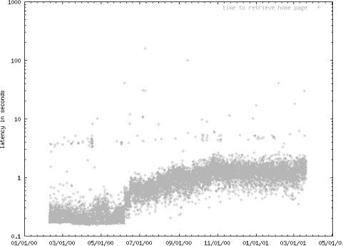
One small problem with this approach is clear if you repeatedly get the same page and look closely at the timings. The first time you get a page it takes about 200 milliseconds longer than each subsequent access using the same Perl process. I attribute this to Perl’s need to create the appropriate objects to hold the request and response. Once it has done that, it doesn’t need to do it again.
Instead of running from cron, you can turn your monitoring script into a functional test by popping up each page in a Netscape browser as you get it, so you can see monitoring as it happens, and also visually verify that pages are correct in addition to checking for a particular string on the page in Perl. For example, from within Perl, you can pop up the http://patrick.net/ page in Netscape like this:
system "netscape -remote 'openURL(http://patrick.net)'";
You can redirect the browser display to any Unix machine running the X Window System, or any Microsoft Windows machine using an X Windows server emulator like Exceed. Controlling Netscape from a script is described at http://home.netscape.com/newsref/std/x-remote.html.
Here is a listing of all the pieces you need to use Perl to monitor your web site. It takes work to get and compile each piece, but once you have them, you have enormous power to write many kinds of monitoring and load testing scripts. I know that compiling in the following order works, but some other orders might work as well. Except for gcc and Perl, these pieces are all available on my web site at http://patrick.net/software/. Perl is available from http://www.perl.com/ and gcc is available from ftp://prep.ai.mit.edu/ as well as many other sites around the world.
gcc
perl 5.004_04 or better
openssl-0.9.4
Crypt-SSLeay-0.15
Time-HiRes-01.20
MIME-Base64-2.11
URI-1.03
HTML-Parser-2.23
libnet-1.0606
Digest::MD5-2.07
libwww.perl-5.44
gnuplot
Now that you know the basics of how to manually write a performance-monitoring script in Perl, I’m going to tell you that you don’t really need to do that. I’ve modified and added to Randal Schwarz’s Perl web proxy server so that it automatically generates monitoring scripts, albeit with some limitations. I call the modified proxy server sprocket. The code is Perl that generates Perl, so it may be hard to follow, but you can download it from http://patrick.net/software/sprocket/sprocket and use it even if you don’t understand exactly how it works.
Here’s how to use it:
First, you’ll need to have the same pieces listed above, all downloadable from http://patrick.net/software/.
Once you have those things installed, get sprocket from http://patrick.net/software/sprocket/sprocket. It is very small and should only take a second or two to download. Put sprocket in a directory from which you can view the resulting PNG images. Your web server’s public_html directory is a good choice.
Now set your web browser’s proxy to the machine sprocket uses by default, port 8008. In Netscape 4, choose Edit → Preferences → Advanced → Proxies → Manual Proxy Configuration → View → HTTP Proxy.
Once your proxy is set, start up sprocket with the -s option for scripting, redirecting the output to the script your want to create. For example:
% sprocket -s > myscript.plYou’ll see feedback on standard error as your script is being created. For example:
# scripting has started (^C when done)
# set your proxy to <URL:http://localhost:8008/>
# then surf to write a script
# scripted a request
# scripted a request
# scripted a request
In this case, we surfed two pages, resulting in three HTTP requests because one of the pages also contained an image. When you have surfed through the pages you want to monitor, enter Ctrl-C to exit sprocket. (If you try to start it up again right away, you may see a “port in use” error, but that should go away in a minute or so.)
Now myscript.pl contains a script that will duplicate nearly verbatim what you did when you were surfing. The exception is that sprocket will not record Set-Cookie responses, because these are unique to the session you had when you were recording the script. The myscript.pl you just created will listen for new Set-Cookie responses when you run it, so you will have a new session each time you run the script you made. Here is the example myscript.pl file we just created:
#!/usr/bin/perl
use Socket;
use Time::HiRes 'time','sleep';
$proto = getprotobyname('tcp');


#vvvvvvvvvvvvvvvvvvvvvvvvvvvvvvvvvvvvvvvvvvvvvvvvvvvvvvvvvvvv
$host   = "vahe";
$port   = 80;
$request = 'GET / HTTP/1.0
Accept: image/gif, image/x-xbitmap, image/jpeg, image/pjpeg, image/png, */*
Accept-Charset: iso-8859-1,*,utf-8
Accept-Encoding: gzip
Accept-Language: en
Host: vahe
User-Agent: sprocket/0.10
Proxy-Connection: Keep-Alive


';
$proof  = 'HTTP/1.1 200 OK';

$request            =~ s|[\r\n]*$|\r\n|; # strip extra \r\n
foreach(@cookies) {
   $request        .= "Cookie: $_\r\n"; # tack on cookies
}
$request           .= "\r\n";           # terminate request with blank line

socket(SOCK, PF_INET, SOCK_STREAM, $proto);
$start              = time(  );
$iaddr              = gethostbyname($host);
$paddr              = sockaddr_in($port, $iaddr);
connect(SOCK, $paddr);
$old_fh             = select(SOCK);     # save the old fh
$|                 = 1;                # turn off buffering
select($old_fh);                         # restore

print SOCK $request;

@response           = <SOCK>;
$end                = time(  );

$path               = $request;
$path               =~ m|^[A-Z]* (.*) HTTP|;
$path               = $1;
$file               = $path;
$file               =~ s|/|_|g;

open(FILE, ">>$file") || die "cannot create file";
$date = `date +'%m %d %H %M %S %Y'`;
chop $date;

# validate response here
if (grep(/$proof/, @response)) {
   print FILE $date, " ", $end - $start, "\n";

}
else {
   print FILE $date, " -1\n";
}

close FILE;

$gnuplot_cmd = qq|
   set term png color
   set output "$file.png"
   set xdata time
   set ylabel "latency in seconds"
   set bmargin 3
   set logscale y
   set timefmt "%m %d %H %M %S %Y"
   plot "$file" using 1:7 title "$path" with lines
|;

open(GP, "|/usr/local/bin/gnuplot");
print GP $gnuplot_cmd;
close(GP);

foreach (@response) {
   /Set-Cookie: (.*)/ && push(@cookies, $1);
}

print;
close(SOCK);
#^^^^^^^^^^^^^^^^^^^^^^^^^^^^^^^^^^^^^^^^^^^^^^^^^^^^^^^^^^^


#vvvvvvvvvvvvvvvvvvvvvvvvvvvvvvvvvvvvvvvvvvvvvvvvvvvvvvvvvvvv
$host   = "vahe";
$port   = 80;
$request = 'GET /webpt_sm.gif HTTP/1.0
Accept: image/gif, image/x-xbitmap, image/jpeg, image/pjpeg, image/png
Accept-Charset: iso-8859-1,*,utf-8
Accept-Encoding: gzip
Accept-Language: en
Host: vahe
Referer: http://vahe/
User-Agent: sprocket/0.10
Proxy-Connection: Keep-Alive


';
$proof  = 'HTTP/1.1 200 OK';

$request            =~ s|[\r\n]*$|\r\n|; # strip extra \r\n
foreach(@cookies) {
   $request        .= "Cookie: $_\r\n"; # tack on cookies
}
$request           .= "\r\n";           # terminate request with blank line

socket(SOCK, PF_INET, SOCK_STREAM, $proto);
$start              = time(  );
$iaddr              = gethostbyname($host);
$paddr              = sockaddr_in($port, $iaddr);
connect(SOCK, $paddr);
$old_fh             = select(SOCK);     # save the old fh
$|                  = 1;                # turn off buffering
select($old_fh);                         # restore

print SOCK $request;

@response           = <SOCK>;
$end                = time(  );

$path               = $request;
$path               =~ m|^[A-Z]* (.*) HTTP|;
$path               = $1;
$file               = $path;
$file               =~ s|/|_|g;

open(FILE, ">>$file") || die "cannot create file";
$date = `date +'%m %d %H %M %S %Y'`;
chop $date;

# validate response here
if (grep(/$proof/, @response)) {
   print FILE $date, " ", $end - $start, "\n";
}
else {
   print FILE $date, " -1\n";
}

close FILE;

$gnuplot_cmd = qq|
   set term png color
   set output "$file.png"
   set xdata time
   set ylabel "latency in seconds"
   set bmargin 3
   set logscale y
   set timefmt "%m %d %H %M %S %Y"
   plot "$file" using 1:7 title "$path" with lines
|;

open(GP, "|/usr/local/bin/gnuplot");
print GP $gnuplot_cmd;
close(GP);

foreach (@response) {
   /Set-Cookie: (.*)/ && push(@cookies, $1);
}

print;
close(SOCK);
#^^^^^^^^^^^^^^^^^^^^^^^^^^^^^^^^^^^^^^^^^^^^^^^^^^^^^^^^^^^


#vvvvvvvvvvvvvvvvvvvvvvvvvvvvvvvvvvvvvvvvvvvvvvvvvvvvvvvvvvvv
$host   = "vahe";
$port   = 80;
$request = 'GET /specs/index.html HTTP/1.0
Accept: image/gif, image/x-xbitmap, image/jpeg, image/pjpeg, image/png, */*
Accept-Charset: iso-8859-1,*,utf-8
Accept-Encoding: gzip
Accept-Language: en
Host: vahe
Referer: http://vahe/
User-Agent: sprocket/0.10
Proxy-Connection: Keep-Alive


';
$proof  = 'HTTP/1.1 200 OK';

$request            =~ s|[\r\n]*$|\r\n|; # strip extra \r\n
foreach(@cookies) {
   $request        .= "Cookie: $_\r\n"; # tack on cookies
}
$request           .= "\r\n";           # terminate request with blank line

socket(SOCK, PF_INET, SOCK_STREAM, $proto);
$start             = time(  );
$iaddr              = gethostbyname($host);
$paddr              = sockaddr_in($port, $iaddr);
connect(SOCK, $paddr);
$old_fh             = select(SOCK);     # save the old fh
$|                  = 1;                # turn off buffering
select($old_fh);                         # restore

print SOCK $request;

@response           = <SOCK>;
$end                = time(  );

$path               = $request;
$path               =~ m|^[A-Z]* (.*) HTTP|;
$path               = $1;
$file               = $path;
$file               =~ s|/|_|g;

open(FILE, ">>$file") || die "cannot create file";
$date = `date +'%m %d %H %M %S %Y'`;
chop $date;

# validate response here
if (grep(/$proof/, @response)) {
   print FILE $date, " ", $end - $start, "\n";
}
else {
   print FILE $date, " -1\n";
}

close FILE;

$gnuplot_cmd = qq|
   set term png color
   set output "$file.png"
   set xdata time
   set ylabel "latency in seconds"
   set bmargin 3
   set logscale y
   set timefmt "%m %d %H %M %S %Y"
   plot "$file" using 1:7 title "$path" with lines
|;

open(GP, "|/usr/local/bin/gnuplot");
print GP $gnuplot_cmd;
close(GP);

foreach (@response) {
   /Set-Cookie: (.*)/ && push(@cookies, $1);
}

print;
close(SOCK);
#^^^^^^^^^^^^^^^^^^^^^^^^^^^^^^^^^^^^^^^^^^^^^^^^^^^^^^^^^^^
You can see that the generated script is low-level and contains no subroutines. It is also very repetitive. But these attributes make it very easy to customize. Note that you cannot record an SSL session (unless the user gives permission), because snooping on an SSL session from a proxy would be proof that SSL doesn’t work! But with some effort, you could turn off SSL on your web server, record a session, then modify your generated myscript.pl to use SSL.
The monitoring script will log a timestamp
and a latency reading for each item it requests, and automatically
generate a graph of the results. The log and graph will appear in the
directory sprocket is in. The name of the log file
will be the path of the URL with each slash (/)
replaced by an underscore (_). The name of the
graph will be the name of the log file, but with
.png appended.
The first time you run the monitoring script, gnuplot will give a warning that you have only one point on each graph so that it does not know how to adjust the axes. You can ignore this warning.
The normal thing to do with your monitoring data is to keep it in a file, but you may want to keep it in a relational database instead. It takes a bit more work to set up, and relational data is not as easily accessible as data in files, but the advantages are huge:
First, you have all of your data in one place, so you don’t have to go hunting for files when you need to find out what happened to the performance of a particular page when a new feature was introduced last month. Of course, having all the data in one place also makes you more vulnerable to losing it all at once.
You have ease of querying. Rather than manually poking or grepping through a huge file, you can simply make SQL queries for the time range in which you’re interested.
SQL has built-in math functions for relatively easy comparisons and manipulation of the data.
If you can connect to the database over a network, you have access to the data remotely, which is not necessarily true for flat files.
If you’re using Perl for monitoring, you should try the Perl DBI (Database Interface) for storing data. You’ll need to download and install the Perl DBI package and a driver for your database. Here’s some example Perl code to do the database insertion.
Instead of doing this, as in the previous script:
print FILE $date, " ", $end - $start, "\n";
You could do the following, assuming that you have a table defined
called perfdata, which has fields for a URL, a
timestamp, and a latency:
use DBI;
$dbh = DBI->connect("dbi:Oracle:perf", "patrick", "passwd")
   or die "Can't connect to Oracle: $DBI::errstr\n";

$sth = $dbh->prepare("insert into perfdata values
   ('$url', to_date('$yyyy $mon $dd $hh $mm $ss', 'YYYY MM DD HH24 MI SS'), $end -
$start)");

$sth->execute(  );
$dbh->disconnect or warn "Disconnect failed: $DBI::errstr\n";
One problem with monitoring data is there is just so much of it, and there is always more. It becomes rather like a memory leak on disk after a while. One way of coping with the volume of data is to simply not log values that are very close to zero. This cuts out most of the data. Another strategy is to roll up daily data into a weekly average after it is a month old, and roll up weekly data into monthly averages after it is a year old, etc. This is the approach taken by the “Big Brother” freeware monitoring tool.
Once you have the data in the database, you’ll want to use it. Here is an example of how to use it to get today’s data out of the database and graph it:
#!/usr/local/bin/perl
use DBI;
$dbh = DBI->connect("dbi:Oracle:perf", "patrick", "passwd")
   or die "Can't connect to Oracle: $DBI::errstr\n";

$url = "/home.html";
$sth = $dbh->prepare("select timestamp, latency from latency where
trunc(timestamp)=trunc(sysdate) and url=$url");
$sth->execute(  );

$gnuplot_cmd = qq|
   set term png color
   set output "$url.png"
   set xdata time
   set ylabel "latency in seconds"
   set bmargin 3
   set logscale y
   set timefmt "%m %d %H %M %S %Y"
   plot "-" using 1:7 title "$path" with lines
|;

while(($timestamp, $latency) = $sth->fetchrow_array) {
   $gp_cmd .= "$timestamp $latency\n";
}

$gp_cmd .= "e\n";

$sth->finish(  );
$dbh->disconnect or warn "disconnect failed: $DBI::errstr\n";

open(GP, "|/usr/local/bin/gnuplot");
print GP $gp_cmd;
close(GP);rstat is an RPC client program I wrote to get and print statistics from any machine running the rpc.rstatd daemon, its server-side counterpart. The rpc.rstad daemon has been used for many years by tools such as Sun’s perfmeter and the rup command. The rstat program is simply a new client for an old daemon. The fact that the rpc.rstatd daemon is already installed and running on most Solaris and Linux machines is a huge advantage over other tools that require the installation of custom agents.
My rstat client compiles and runs on Solaris and Linux as well and can get statistics from any machine running a current rpc.rstatd daemon, such as Solaris, Linux, AIX, and OpenBSD. The rpc.rstatd daemon is started from /etc/inetd.conf on Solaris. I will probably also port the rstat client to other platforms. It is similar to vmstat, but has some advantages over vmstat:
The fact that it runs remotely means that
you can use a single central machine to monitor the performance of
many remote machines. It also has a disadvantage in that it does not
give the useful scan rate measurement of memory shortage, the
sr column in vmstat.
rstat will not work across most firewalls because
it relies on port 111, the RPC port, which is usually blocked by
firewalls.
You can download rstat from http://patrick.net/software/rstat/rstat.html. As mentioned earlier, Sun’s perfmeter program is also an rpc.rstatd client and can also log remote server statistics to a file. However, I haven’t managed to run perfmeter without its GUI, though it could perhaps be done using Xvfb, the X virtual frame buffer.
To use rstat, simply
give it the name or IP address of the machine you wish to monitor.
Remember that rpc.rstatd must be running on that
machine. The rup command is extremely useful here
because with no arguments, it simply prints out a list of all
machines on the local network that are running the
rstatd demon. If a machine is not listed, you may
have to start rstatd manually. To start
rpc.rstatd under Red Hat Linux, run
/etc/rc.d/init.d/rstatd start as
root. On Solaris, first try running the
rstat client because inetd is
often already configured to automatically start
rpc.rstatd on request. If it the client fails with
the error “RPC: Program not
registered,” make sure you have this line in your
/etc/inet/inetd.conf and kill
-HUP your inetd process to get it to
re-read inetd.conf, as follows:
rstatd/2-4 tli rpc/datagram_v wait root /usr/lib/netsvc/rstat/rpc.rstatd rpc.rstatd
Then you can monitor that machine like this:
% rstat enkidu
2001 07 10 10 36 08  0   0   0 100    0    27   54     1     0    0   12  0.1
This command will give you a one-second average and then it will exit. If you want to continuously monitor, give an interval in seconds on the command line. Here’s an example of one line of output every two seconds:
% rstat enkidu 2
2001 07 10 10 36 28  0   0   1  98    0     0    7     2     0    0   61  0.0
2001 07 10 10 36 30  0   0   0 100    0     0    0     2     0    0   15  0.0
2001 07 10 10 36 32  0   0   0 100    0     0    0     2     0    0   15  0.0
2001 07 10 10 36 34  0   0   0 100    0     5   10     2     0    0   19  0.0
2001 07 10 10 36 36  0   0   0 100    0     0   46     2     0    0  108  0.0
^C
To get a usage message, the output format, the version number, and
where to go for updates, just type rstat with
no parameters:
% rstat
usage: rstat machine [interval]
output:
yyyy mm dd hh mm ss usr wio sys idl pgin pgout intr ipkts opkts coll  cs load
docs and src at http://patrick.net/software/rstat/rstat.html
Notice that the column headings line up with the output data.
The output
may look meaningless to the uninitiated, but it is quite useful and
the format was chosen to be easily plotted by the
gnuplot graphing program. You may download
gnuplot from http://www.gnuplot.org/ or http://patrick.net/software/. You can ask
gnuplot to choose any of the fields for plotting.
To create a graph of your rstat data, redirect or
save the rstat output data in a file, which
I’ve named rstat.out here. Then
create the following gnuplot configuration file,
which we name enkidu.gp. Then just run
gnuplot enkidu.gp and
gnuplot will create a PNG file called
enkidu.png that is suitable for display on a web
site:
set term png color
set output "enkidu.png"
set xdata time
set timefmt "%Y %m %d %H %M %S"
set bmargin 3
set y2label "load"
set ylabel "context switching"
set ytics nomirror
set y2tics nomirror
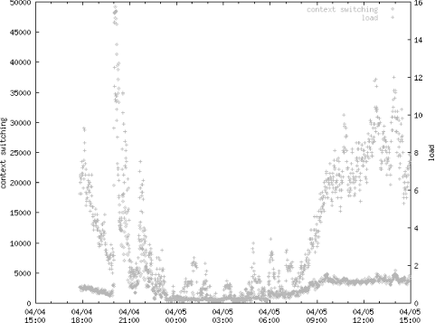
plot "rstat.out" using 1:17 axes x1y1 title "context switching", \
"rstat.out" using 1:18 axes x1y2 title "load"Figure 4-2 shows an example GIF depicting context switching and load (the 17th and 18th fields) that I created with rstat and gnuplot.
As with latency data, it is good to store rstat data in a database for later retrieval and correlation with problems. Here’s a SQL command that can be used to create a table for rstat data in Oracle:
create table rstat (
    machine     varchar2(20),
    timestamp   date not null,
    usr         number(3),
    wio         number(3),
    sys         number(3),
    idl         number(3),
    pgin        number(6),
    pgout       number(6),
    intr        number(6),
    ipkts       number(6),
    opkts       number(6),
    coll        number(6),
    cs          number(8),
    load        number(3,1)
    )/
And here’s some example Perl code to run rstat, parse out the fields, and perform the database insertion:
#!/usr/local/bin/perl
use DBI;
$machine = "vatche";
$interval = 60;
$dbh     = DBI->connect("dbi:Oracle:perf", "patrick", "passwd")
               or die "Can't connect to Oracle: $DBI::errstr\n";

open(RSTAT, "rstat $machine $interval |") || die "could not start rstat";

while(<RSTAT>) {
       ($yyyy, $mon, $dd, $hh, $mm, $ss, $usr, $wio, $sys, $idl, $pgin, $pgout,
$intr,
       $ipkts, $opkts, $coll, $cs, $load) = split(/\s+/);
       $sth = $dbh->prepare("insert into rstat values
                 ('$machine', to_date('$yyyy $mon $dd $hh $mm $ss', 'YYYY MM DD HH24
MI SS'),
                 $usr, $wio, $sys, $idl, $pgin, $pgout, $intr, $ipkts, $opkts, $coll,
$cs, $load)");
       $sth->execute(  );
}

# If rstat dies, at least we should try to disconnect nicely.
$dbh->disconnect or warn "Disconnect failed: $DBI::errstr\n";Now that you have system data in your database, how do you use it? The answer is any way that you use any other kind of relational data. Let’s say you want to get the average of the system and user CPU usage for October 8, 2001, between the hours of 9 a.m. and 4 p.m. Here is a query that does this:
select avg(sys + usr) from rstat where timestamp between
to_date('2001 10 08 09', 'YYYY MM DD HH24') and
to_date('2001 10 08 16', 'YYYY MM DD HH24') and
machine='mars';Often it is useful to be able to grep, sort, or otherwise process database data on the Unix command line, but most SQL querying tools are “captive user interfaces” that do not play nicely with Unix standard in and standard out. Here is a simple Perl script that will let you do that if you have the DBI module installed and are using Oracle. It’s called sql.pl and is available at http://patrick.net/software/.
#!/usr/local/bin/perl

use DBI;

$ENV{ORACLE_HOME} = "/path/to/ORACLE/product";

$dbh = DBI->connect("dbi:Oracle:myinstance", "mylogin", "mypassword")
or die "Can't connect to Oracle: $DBI::errstr\n";

$sql = $ARGV[0];
$sth = $dbh->prepare($sql);
$sth->execute(  );

while(@row = $sth->fetchrow_array) {
   print "@row\n";
}

$sth->finish(  );
$dbh->disconnect or warn "Disconnect failed: $DBI::errstr\n";Getting a single number is interesting, but it is more interesting to see how data varies over time. The following is the HTML for a CGI that will allow anyone to view graphs of your collected rstat data. It will graph a single parameter over time. You will need to alter it to reflect your ORACLE_HOME, your Oracle user and password, and your machine names, but aside from that, it should be ready to run. You can download this script from http://patrick.net/software/graph.cgi.
#!/usr/local/bin/perl
#Author: Patrick Killelea
#Date:  12 April 2001

# You will need to replace "myinstance", "mylogin", and "mypassword" below with
# values for your own environment.

use DBI;

$ENV{ORACLE_HOME} = "/opt/ORACLE/product";

print qq|Content-type: text/html\n\n|;

print qq|<HTML><HEAD><TITLE>generate a graph</TITLE>
<meta http-equiv = "Pragma" Content = "no-cache">
<meta http-equiv = "Expires" Content = "Thu, Jan 1 1970 12:00:00 GMT">
</HEAD><BODY><H1>generate a graph</H1>|;

if ($ENV{'REQUEST_METHOD'} eq 'POST') {
   read(STDIN, $buffer, $ENV{'CONTENT_LENGTH'});
   @pairs = split(/&/, $buffer);
   foreach $pair (@pairs) {
       ($name, $value) = split(/=/, $pair);

       $value  =~ tr/+/ /;
       $value  =~ s/%([a-fA-F0-9][a-fA-F0-9])/pack("C", hex($1))/eg;
       $contents{$name} = $value;
   }
}

$machine  = $contents{"machine"};
$parameter = $contents{"parameter"};
$daterange = $contents{"daterange"};

if ($machine && $parameter && daterange) {

   `/bin/rm tmp/*.gif`;

   $dbh = DBI->connect("dbi:Oracle:myinstance", "mylogin", "mypassword")
        or die "Can't connect to Oracle: $DBI::errstr\n";

   $sql  = "select to_char(timestamp, 'YYYY MM DD HH24 MI'), $parameter from rstat ";

   if ($daterange eq "today") {
       $sql .= "where timestamp between trunc(sysdate) and sysdate and
machine='$machine' ";
   }

   if ($daterange eq "yesterday") {
       $sql .= "where timestamp between trunc(sysdate) - 1 and trunc(sysdate) and
machine='$machine'";
   }

   if ($daterange eq "t-7") {
       $sql .= "where timestamp between trunc(sysdate) - 7 and sysdate and
machine='$machine'";
   }

   if ($daterange eq "t-30") {
       $sql .= "where timestamp between trunc(sysdate) - 30 and sysdate and
machine='$machine'";
   }

   if ($daterange eq "t-365") {
       $sql .= "where timestamp between trunc(sysdate) - 365 and sysdate and
machine='$machine'";
   }

   $sth = $dbh->prepare($sql);
   $sth->execute(  ) || print $dbh->errstr;

   ($timestamp, $item) = $sth->fetchrow_array; # get one sample row to be sure we
have data

   if ($timestamp) {

       $date = `date`;
       chop $date;

       open(GP, "|/usr/local/bin/gnuplot");
       print GP $gp_cmd;
       print GP qq|
           set xdata time
           set timefmt "%Y %m %d %H %M"
           set term gif
           set xlabel "graph made on $date"
           set bmargin 4
           set ylabel "$parameter"
           set output "tmp/$$.gif"
           plot '-' using 1:6 title "$parameter on $machine" with lines lt 2
       |;

       while(($timestamp, $item) = $sth->fetchrow_array) {
           print GP "$timestamp $item\n";
       }

       print GP "e\n";
       close(GP);

       $sth->finish(  );
       $dbh->disconnect or warn "acsiweba disconnect failed: $DBI::errstr\n";

       print "<p><img src=\"tmp/$$.gif\"><p>";
       print "graph was generated from this query:<p> $sql\n";
   }
   else {
       print "Sorry, I do not have the requested data for that time range for
$machine.";
   }
}

print qq|
<FORM
METHOD="POST" ENCTYPE="application/x-www-form-urlencoded">
<P>select a machine
<SELECT NAME="machine">
<OPTION SELECTED VALUE="venus">venus database
<OPTION VALUE="mars">mars backup database
<OPTION VALUE="pluto">pluto middleware
<OPTION VALUE="saturn">saturn nfs
<OPTION VALUE="earth">earth middleware
</SELECT>
</P>
<P>select a parameter
<SELECT NAME="parameter">
<OPTION SELECTED VALUE="usr">user cpu
<OPTION VALUE="wio">wait io cpu
<OPTION VALUE="sys">system cpu
<OPTION VALUE="idl">idle cpu
<OPTION VALUE="pgin">pgs in per second
<OPTION VALUE="pgout">pgs out per second
<OPTION VALUE="intr">interrupts per second
<OPTION VALUE="ipkts">network in pkts per second
<OPTION VALUE="opkts">network out pkts per second
<OPTION VALUE="coll">collisions per second
<OPTION VALUE="cs">context switches per second
<OPTION VALUE="load">load: procs waiting to run
</SELECT>
</P>
<P>select a date range
<SELECT NAME="daterange">
<OPTION SELECTED VALUE="today">today
<OPTION VALUE="yesterday">yesterday
<OPTION VALUE="t-7">last 7 days
<OPTION VALUE="t-30">last 30 days
<OPTION VALUE="t-365">last 365 days
</SELECT>
</P>
<P>
<INPUT TYPE="submit" NAME="graph" VALUE="graph">
</P><HR><P>|;

print qq|</FORM>Questions? Write
<A HREF="mailto:p\@patrick.net">p\@patrick.net</A>
</BODY></HTML>|;It is very valuable to know which processes are using the most CPU time or other resources on a remote machine. The rpc.rstatd daemon, which we used earlier, does not provide per-process information. Commercial software, such as Measureware, requires the installation of potentially buggy remote agents to report per-process information, and keeps its data in a proprietary format. It is often unacceptable to install unknown agents on important production machines, and it is never to your advantage to have your data locked into a proprietary format. Here we look at alternate freeware for collecting the same data—first, at a web server, and second, at telnet from a Perl script.
It is not hard to create a CGI that calls ps, vmstat, sar, top, or other system monitoring programs that were intended to be used only by someone logged in to that machine. For example, using Apache, you could copy /bin/ps to /home/httpd/cgi-bin/nph-ps and suddenly you have a version of ps that is directly runnable from the Web.
You need to rename it with the nph- prefix to tell the Apache web server not to expect or add any headers. If you don’t, the web server will expect a Content-Type header from ps and give an error because ps does not output that header. The nph- header tells Apache not to worry about it. (“nph” stands for “nonparsed headers.”) What you then get will not be prettily formatted in a browser, but at least will be usable by a script that calls that URL. You could also write a CGI that in turn calls ps, then adds the appropriate header, and does any other processing you like, but this adds the overhead of yet another new process every time you call it.
I have used a very tiny web server called mathopd from http://www.mathopd.org/ to run ps as a CGI. There is essentially no documentation of this web server, which is distributed as source code, but it is simple enough. It compiles cleanly on Linux, but requires a few tweaks to compile on Solaris, where it also needs the -lnsl and -lsocket options to gcc in the Makefile. mathopd has the advantage that it is even smaller than Apache, runs as a single process, and does not allocate any new memory after startup. I am reasonably confident that mathopd is free of memory leaks, but it is simple to write a cron job that kills and restarts it each night if this is a concern. It is single-process and single-threaded. If you write its log files to /dev/null, it should not use any disk space. I keep a compiled copy on my web site at http://patrick.net/software/.
Here is a script that watches CPU usage, and if idle time falls below a certain threshold, it hits the URL to run ps as a CGI and mail the result to an administrator, who can determine which of the processes is the offender. It can be run as a cron job, or you can make it into a loop and leave a single process going. (I prefer a cron job because long-running jobs tend to leak memory or get killed.)
#!/usr/local/bin/perl
use LWP::UserAgent;

$thresh  = 50;                # usr CPU threshold, above which we report top 10 procs
$machine = www.patrick.net;
$\       = "\n";              # automatically append newline to print statements

# grab the cpu usage
$_       = `/opt/bin/rstat $machine`;

($yyyy, $mon, $dd, $hh, $mm, $ss, $usr, $wio, $sys, $idl, $pgin, $pgout, $intr,
$ipkts, $opkts, $coll, $cs, $load) = split(/\s+/);

if ($idl < $thresh) {
   print "$machine is under $thresh\n";
   $ua = LWP::UserAgent->new;

   $request = new HTTP::Request('GET', "http://$machine/nph-ps");
   $response = $ua->request($request);

   if (!$response->is_success) {
       die $request->as_string(  ), " failed: ", $response->error_as_HTML;
   }

   open (MAIL, '|/bin/mail hostmaster@bigcompany.com');
   print MAIL 'From: hostmistress@bigcompany.com';
   print MAIL 'Reply-To: hostmistress@bigcompany.com';
   print MAIL "Subject: $machine CPU too high";
   print MAIL "";
   print MAIL "CPU idle time is less than $thresh\% on $machine";
   print MAIL "Here are the top 10 processes by CPU on $machine";
   print MAIL $response->content;
   print MAIL "\nThis message generated by cron job /opt/bin/watchcpu.pl";
   close MAIL;
}The problem with running a web server to report performance statistics is that it requires the installation of software on your production systems. Installation of extra software on production systems should be avoided for many reasons. Extra software may leak memory or otherwise use up resources, it may open security holes, and it may just be a pain to do. Fortunately, all you really need for a pretty good monitoring system is permission to use tools and interfaces that are probably already there, such as the rstat daemon, SQL, SNMP, and Telnet. They will not work through a firewall the way web server-based tools do, but your monitoring system should be on the secure side of your firewall in most cases anyway.
Telnet is the most flexible of these interfaces, because a Telnet session can do anything a user can do. Here is an example script that will log in to a machine given on the command line, run ps, and dump the results to standard output:
#!/usr/local/bin/perl

use Net::Telnet;

$host = $ARGV[0];
$user = "patrick";
$password = "passwd";

my $telnet = Net::Telnet->new($host);
$telnet->login($user, $password);
my @lines = $telnet->cmd('/usr/bin/ps -o pid,pmem,pcpu,nlwp,user,args');
print @lines;
$telnet->close;
This ability to run a command from Telnet and use the results in a Perl script is incredibly useful, but also easily abused, for example, by running many such scripts every minute from cron jobs. Every login will take a tiny bit of disk space (for instance, each will be recorded in /var/run/utmp on Linux.) Please be cautious about how much monitoring you are doing, lest you become part of your own performance problem.
To fill out a per-process monitoring system with telnet and ps, we would like to be able to store our data in a relational database. For that, we need to define a database table. Here’s the definition of a table for storing ps data in Oracle that I use to store data coming from the Solaris command /usr/bin/ps -o pid,pmem,pcpu,nlwp,user,args:
create table ps(
   machine    varchar2(20),
   timestamp  date not null,
   pid        number(6),
   pmem       number(3,1),
   pcpu       number(3,1),
   nlwp       number(5),
   usr        varchar2(8),
   args       varchar2(24)
);
And here’s a Perl script that can telnet to various machines, run ps, and store the resulting ps data in a database:
#!/usr/local/bin/perl

$ENV{ORACLE_HOME} = "/opt/ORACLE/product";

use DBI;
use Net::Telnet;

$user      = "patrick";
$pwd       = "telnetpasswd";

$machine = $ARGV[0];

my $telnet = Net::Telnet->new($machine);
$telnet->timeout(45);
$telnet->login($user,$pwd);
my @lines = $telnet->cmd('/usr/bin/ps -e -o pid,pmem,pcpu,nlwp,user,args');
$telnet->close;

$dbh = DBI->connect("dbi:Oracle:acsiweba", "patrick", "dbpasswd")
   or die "Can't connect to Oracle: $DBI::errstr\n";

foreach (@lines) {
   # Grab the lines with "dummy" in them, and parse out this data:
   #     PID      %MEM      %CPU   NLWP   USER         COMMAND
   #
   # and insert the fields into ps table, which looks like this:
   #
   # Name                                      Null?   Type
   # -------------------------------------------------------
   # MACHINE                                            VARCHAR2(20)
   # TIMESTAMP                                 NOT NULL DATE
   # PID                                                NUMBER(6)
   # PMEM                                               NUMBER(3,1)
   # PCPU                                               NUMBER(3,1)
   # NLWP                                               NUMBER(5)
   # USR                                                VARCHAR2(8)
   # ARGS                                               VARCHAR2(24)

   if (/(\d+) +(\d+\.\d) +(\d+\.\d) +(\d+) +(\w+) .*Didentifier=(\w+)/) {

       $sth = $dbh->prepare("insert into ps values ('$machine', sysdate, '$1', '$2',
'$3', '$4', '$5', '$6')");
       $sth->execute(  );
   }
}

$dbh->disconnect or warn "Disconnect failed: $DBI::errstr\n";Now that we have all this wonderful ps data in a database, what are we going to do with it? Why, generate graphs of it on request, of course, just like we did with the rstat data. Here’s a sample CGI script that will do just that, and a sample graph generated from it. (To use the CGI script, you have to put it in your web server’s cgi-bin directory, and then hit the URL corresponding to the script.)
#!/usr/local/bin/perl
use DBI;
$ENV{ORACLE_HOME} = "/opt/ORACLE/product";
print qq|Content-type: text/html\n\n|;
#<meta http-equiv = "Pragma" Content = "no-cache">
#<meta http-equiv = "Expires" Content = "Thu, Jan 1 1970 12:00:00 GMT">
print qq|<HTML><HEAD><TITLE>generate a graph</TITLE>
</HEAD><BODY><H1>generate a graph</H1>|;
if ($ENV{'REQUEST_METHOD'} eq 'POST') {
read(STDIN, $buffer, $ENV{'CONTENT_LENGTH'});
@pairs = split(/&/, $buffer);
foreach $pair (@pairs) {
($name, $value) = split(/=/, $pair);
$value =~ tr/+/ /;
$value =~ s/%([a-fA-F0-9][a-fA-F0-9])/pack("C", hex($1))/eg;
$contents{$name} = $value;
}
}
$machine = $contents{"machine"};
$args = $contents{"args"};
$daterange = $contents{"daterange"};
$parameter = $contents{"parameter"};
if ($machine && $parameter && daterange) {
`/bin/rm tmp/*.gif`; # possible removal of someone else's gif before they saw it
$dbh = DBI->connect("dbi:Oracle:acsiweba", "patrick", "dbpasswd")
or die "Can't connect to Oracle: $DBI::errstr\n";
$sql = "select to_char(timestamp, 'YYYY MM DD HH24 MI'), $parameter from patrick.
ps ";
if ($daterange eq "today") {
$sql .= "where timestamp between trunc(sysdate) and sysdate and
machine='$machine'";
}
if ($daterange eq "yesterday") {
$sql .= "where timestamp between trunc(sysdate) - 1 and trunc(sysdate) and
machine='$machine'";
}
if ($daterange eq "t-7") {
$sql .= "where timestamp between trunc(sysdate) - 7 and sysdate and
machine='$machine'";
}
if ($daterange eq "t-30") {
$sql .= "where timestamp between trunc(sysdate) - 30 and sysdate and
machine='$machine'";
}
if ($daterange eq "t-365") {
$sql .= "where timestamp between trunc(sysdate) - 365 and sysdate and
machine='$machine'";
}
$sql .= " and args='$args'";
#print "<p>start of query ", `date`;
$sth = $dbh->prepare($sql);
$sth->execute( ) || print $dbh->errstr;
($timestamp, $item) = $sth->fetchrow_array; # get one sample row to be sure we
have data
if ($timestamp) {
#print "<p>end of query ", `date`;
$date = `date`;
chop $date;
open(GP, "|/usr/local/bin/gnuplot");
print GP $gp_cmd;
print GP qq|
set xdata time
set timefmt "%Y %m %d %H %M"
set term gif
set xlabel "graph made on $date"
set bmargin 4
set ylabel "$parameter"
set output "tmp/$$.gif"
plot '-' using 1:6 title "$args $parameter on $machine" with lines lt 2
|;
while(($timestamp, $item) = $sth->fetchrow_array) {
print GP "$timestamp $item\n";
}
print GP "e\n";
close(GP);
$sth->finish( );
$dbh->disconnect or warn "acsiweba disconnect failed: $DBI::errstr\n";
#print "<p>end of plotting ", `date`;
print "<p><img src=\"tmp/$$.gif\"><p>";
print "graph was generated from this query:<p> $sql\n";
}
else {
print "Sorry, I do not have the requested data for that time range for
$machine.";
}
}
print qq|
<FORM
METHOD="POST" ENCTYPE="application/x-www-form-urlencoded">
<P>select a machine
<SELECT NAME="machine">
<OPTION SELECTED VALUE="mars">mars middleware
<OPTION VALUE="venus">venus middleware
<OPTION VALUE="mercury">mercury middleware
</SELECT>
</P>
<SELECT NAME="args">
<OPTION SELECTED VALUE="purchase">purchase app
<OPTION VALUE="billing">billing app
<OPTION VALUE="accounting">accounting app
</SELECT>
</P>
<P>select a parameter
<SELECT NAME="parameter">
<OPTION SELECTED VALUE="pmem">pmem
<OPTION VALUE="pcpu">pcpu
<OPTION VALUE="nlwp">nwlp
</SELECT>
</P>
<P>select a date range
<SELECT NAME="daterange">
<OPTION SELECTED VALUE="today">today
<OPTION VALUE="yesterday">yesterday
<OPTION VALUE="t-7">last 7 days
<OPTION VALUE="t-30">last 30 days
<OPTION VALUE="t-365">last 365 days
</SELECT>
</P>
<P>
<INPUT TYPE="submit" NAME="graph" VALUE="graph">
</P><HR><P>|;
print qq|</FORM>Questions? Write
<A HREF="mailto:p\@patrick.net">p\@patrick.net</A>
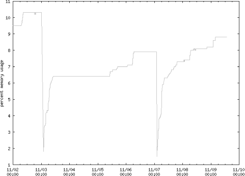
</BODY></HTML>|;Figure 4-3 is an example graph generated from this CGI, showing a memory leak in an application, and restarts on 11/3 and 11/7.
You can also monitor the contents of the web pages rather than the latency. For example, the Weblogic application server gives a password-protected web page showing the number of database connections used at any given time. The page is intended only for a human reader, but knowing how to automatically grab web pages, we can “screen scrape” the Weblogic monitoring page and keep a log of the number of database connections used over each day and plot this log. We can snoop the header containing the base 64 encoding of the user ID and password and then use that in our script. Here’s a simple script that will grab the Weblogic T3AdminJDBC page, parse out the number of connections in use, and log that data to a file:
#!/usr/local/bin/perl

use LWP::UserAgent;
use HTTP::Headers;
use HTTP::Request;
use HTTP::Response;

$gnuplot    = "/usr/local/bin/gnuplot";


MAIN: {
   $ua = LWP::UserAgent->new;
   $ua->timeout(60);          # Set timeout to 60 seconds

   &get("http://$ARGV[0]/T3AdminJDBC");

   s/<.*?>/ /g;               # remove all the HTML tags
   /cxn_pool +(\d+) +(\d+)/;  # grab the relevant line
   &log("cxn_pool", $1, $2);

   `$gnuplot *.gp`;
}

sub get {
   local ($url) = @_;

   $request = new HTTP::Request('GET', "$url");

   # This is the base 64 encoding of the weblogic admin login and password.
   $request->push_header("Authorization" => "Basic slkjSLDkf98aljk98797");

   $response = $ua->request($request);

   if (!$response->is_success) {
       #die $request->as_string(  ), " failed: ", $response->error_as_HTML;
       # HTTP redirections are considered failures by LWP.
   }

   # Put response in default string for easy verification.
   $_ = $response->content;
}

# Write log entry in format that gnuplot can use to create a gif.
sub log {

   local ($file, $connections, $pool) = @_;
   $date = `date +'%Y %m %d %H %M %S'`;
   chop $date;

   # Corresponding to gnuplot command: set timefmt "%Y %m %d %H %M %S";

   open(FH, ">>$file") || die "Could not open $file\n";
   printf FH "$date $connections $pool\n";
   close(FH);
}
Once we have our data file, we can plot it using the following gnuplot configuration file:
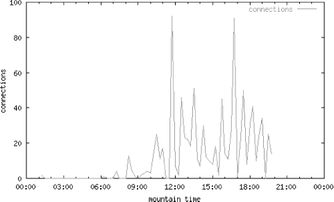
set term png color
set output "connections.gif"

set xdata time
set timefmt "%H %M %S"
set xrange ["00 00 00":"24 00 00"]
set xlabel "mountain time"
set format x "%H:%M"
set bmargin 3
set ylabel "connections"
set yrange [0:100]

plot "connections.log" using 4:7 title "connections" w l lt 3
And the result is a graph like the one in Figure 4-4.
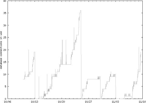
We can also easily store this connection data in a database table itself, as we did with the ps data. Having done that, we can adapt the dynamic graph generation CGI script above to plot connection data. This is very useful for finding “leaks” in database connections — that is, connections that do not get cleaned up after use. This typically happens because of poor or nonexistent error handling, which leaves an unused database connection in limbo. Figure 4-5 is an example CGI-generated graph over 30 days, showing how the database connections build up between restarts of the Weblogic application server. The server was restarted on 10/13, 10/25, 10/30, and 11/3.
Just because I prefer Perl doesn’t mean you have to use Perl. Here is an example Java program that monitors the first edition of this book’s Amazon sales rank. I wrote a Perl program that does the same thing, and Ian Darwin, the author of O’Reilly’s Java Cookbook, showed me that it’s not much harder in Java. Thanks to Ian for the following example:
import java.io.*;
import com.darwinsys.util.FileIO;
import java.net.*;
import java.text.*;
import java.util.*;
import org.apache.regexp.*;

/** Graph of a book's sales rank on a given bookshop site.
* @author Ian F. Darwin, ian@darwinsys.com, Java Cookbook author,
*      translated fairly literally from Perl into Java.
* @author Patrick Killelea <p@patrick.net>: original Perl version,
*      from the 2nd edition of his book "Web Performance Tuning".
* @version $Id: BookRank.java,v 1.10 2001/04/10 00:28:02 ian Exp $
*/

public class BookRank {
       public final static String ISBN = "0937175307";
       public final static String DATA_FILE = "lint.sales";
       public final static String GRAPH_FILE = "lint.png";
       public final static String TITLE = "Checking C Prog w/ Lint";
       public final static String QUERY = "
                       "http://www.quickbookshops.web/cgi-bin/search?isbn=";

       /** Grab the sales rank off the web page and log it. */
       public static void main(String[] args) throws Exception {

               // Looking for something like this in the input:
               //      <b>QuickBookShop.web Sales Rank: </b>
               //      26,252
               //      </font><br>
               // Patrick Killelea's original RE formulation : match number with
               // comma included, just print minus ",". Loses if fall below 100,000.
               RE r = new RE(" Sales Rank: </b>\\s*(\\d*),*(\\d+)\\s");
               // Java: should use "[\d,]+" to extract the number and
               // NumberFormat.getInstance().parse(  ) to convert to int.

               // Open the URL and get a Reader from it.
               BufferedReader is = new BufferedReader(new InputStreamReader(
                       new URL(QUERY + ISBN).openStream(  )));
               // Read the URL looking for the rank information, as
               // a single long string, so can match RE across multi-lines.
               String input = FileIO.readerToString(is);

               // If found, append to sales data file.
               if (r.match(input)) {
                       PrintWriter FH = new PrintWriter(
                               new FileWriter(DATA_FILE, true));
                       String date = // `date +'%m %d %H %M %S %Y'`;
                               new SimpleDateFormat("MM dd hh mm ss yyyy ").
                               format(new Date(  ));
                       // Paren 1 is the optional thousands; paren 2 is low 3 digits.

                       FH.println(date + r.getParen(1) + r.getParen(2));
                       FH.close(  );
               }

               // Whether current data found or not, draw the graph, using
               // external plotting program against all historical data.
               // Could use gnuplot, R, any other math/graph program.
               // Better yet: use one of the Java plotting APIs.

               String gnuplot_cmd =
                       "set term png color\n" +
                       "set output \"" + GRAPH_FILE + "\"\n" +
                       "set xdata time\n" +
                       "set ylabel \"Book sales rank\"\n" +
                       "set bmargin 3\n" +
                       "set logscale y\n" +
                       "set yrange [1:60000] reverse\n" +
                       "set timefmt \"%Y %m %d %H %M %S\"\n" +
                       "plot \"" + DATA_FILE +
                               "\" using 1:7 title \"" + TITLE + "\" with lines\n"
               ;

               Process p = Runtime.getRuntime(  ).exec("/usr/local/bin/gnuplot");
               PrintWriter gp = new PrintWriter(p.getOutputStream(  ));
               gp.print(gnuplot_cmd);
               gp.close(  );
       }
}
And here’s the original in Perl:
#!/usr/local/bin/perl -w

################################
# Set up user agent and proxy. #
################################

use  LWP::UserAgent;
$ua = LWP::UserAgent->new;
$ua->proxy('http', 'http://httpprox:8080');

#######################################################
# Grab the sales rank off the Amazon page and log it.
#######################################################

$url     = "http://www.amazon.com/exec/obidos/ASIN/1565923790/";
$request = new HTTP::Request('GET', "$url");
$response = $ua->request($request);
$_       = $response->content;
m|Amazon.com Sales Rank: </b>\s*(\d*),*(\d+)\s|s && do {
   open(FH, ">>wpt.sales") || die "Could not open wpt.sales\n";
   $date = `date +'%m %d %H %M %S %Y'`;
   chop $date;
   printf FH "%s %s\n", $date, $1.$2;
   close(FH);
};

#########################
# Regenerate the graph. #
#########################

$gnuplot_cmd = qq|
   set term png color
   set output "sales.png"
   set xdata time
   set ylabel "Amazon sales rank"
   set bmargin 3
   set logscale y
   set yrange [1:30000] reverse
   set timefmt "%m %d %H %M %S %Y"
   plot "wpt.sales" using 1:7 title "web performance tuning" with lines
|;

open(GP, "|/usr/local/bin/gnuplot");
print GP $gnuplot_cmd;
close(GP);Once you are updating a few graphs via cron jobs, you may want to set up a PC in a public place to show the constantly updated graphs to those who have an interest. Here’s a bit of HTML to help you do that. It will make a square table with four images:
<html>
<head>
<title>System Dashboard http://patrick.net/graphs.html</title>
<meta http-equiv = "Refresh" Content = "300">
<meta http-equiv = "Pragma" Content = "no-cache">
<meta http-equiv = "Expires" Content = "Thu, Jan 1 1970 12:00:00 GMT">
</head>
<body bgcolor="#ffffff">
<table cols=2>
   <tr>
       <td><IMG SRC="users.png"></td>
       <td><IMG SRC="purchases.png"></td>
   </tr>
   <tr>
       <td><IMG SRC="cpu.png"></td>
       <td><IMG SRC="disk.png"></td>
   </tr>
</table>
</body>
</html>
The 300 is the number of seconds before we refresh
the four graph images. The other
“meta” tags try to defeat the
caching of the browser, which may try to keep the graphs in its cache
rather than refresh them from the web server. If you have more than
four graphs, it is hard to show them all on a single page, so you may
want to alternate between two displays.
<META HTTP-EQUIV = "Refresh" Content = "300;URL=http://patrick.net/moregraphs.html">
If you don’t like the “chrome” — that is, the buttons at the top of the browser — here’s another HTML file, containing a JavaScript way to pop up your dashboard window without any of that:
<html>
<head>
<title>Dashboard Launcher</title>
</head>
<body bgcolor="#ffffff">

<script language="JavaScript">
<!--
function MM_openBrWindow(theURL,winName,features) { //v2.0
   window.open(theURL,winName,features);
}
//-->
</script>

<a href="index.html"
onclick="MM_openBrWindow('graphs.html',
                        '',
                        'width=640,height=480,resizable=1')">
pop
</body>
</html>Monitoring via your web site is good, but too much of a good thing can be bad.
Keynote is a monitoring service that can end up hitting your heavy dynamic pages from all over the U.S. If each of their agents is set to hit it once per minute, 60 agents will cause hits once per second. Resonate, a load balancing system, could also get those pages every second. And you can easily add to the load as well by inadvertently doing too much monitoring. Keep the capacity usage of monitoring systems to a low percentage of your system capabilities.
The Simple Network Management Protocol (SNMP) is a standardized way to track the machines, applications, and bandwidth of your network. It is a valuable tool for performance tuning. SNMP originated in the Unix community, but it is now available on most platforms. There are many SNMP management tools to choose from, such as HP’s OpenView and products from IBM, 3Com, Cabletron, Sun, and Cisco.
You can avoid having SNMP traffic add to your production traffic by setting up a separate SNMP management network, although this can be expensive. Each monitored device or application is referred to as an agent and has a Management Information Base (MIB) that defines the information the agent tracks and what sort of remote control of the agent is allowed.
RMON (Remote MONitoring) is an SNMP MIB definition for Ethernet, defined in RFC 1757 (formerly RFC 1271). RMON II can see HTTP and other kinds of application-level traffic and generate statistics on these. RMON allows monitored devices to be proactive about signalling errors, unlike the traditional polling mechanism used by SNMP. Many commercial systems, such as Tivoli, HP OpenView, and Sun Netmanager understand and use RMON.
The Application Response Measurement API (ARM) provides a standard way to characterize resource consumption by a particular application, even in a distributed environment. It was developed by Hewlett-Packard and Tivoli Systems. It is a good idea, but it requires that software developers instrument their code using this API. To date, few software vendors have released ARM-compliant code. The ARM working group web site is at http://www.cmg.org/.
A few more benchmarking resources on the Web are as follows: the Linpack site, which compares Java to Fortran, at http://www.netlib.org/benchmark/linpackjava/; the Netperf site, which has a large database of network performance results found with the free Netperf tool, at http://www.netperf.org/; and a Java benchmark page at http://www.cs.cmu.edu/~jch/java/benchmarks.html.
Get Web Performance Tuning, 2nd Edition now with the O’Reilly learning platform.
O’Reilly members experience books, live events, courses curated by job role, and more from O’Reilly and nearly 200 top publishers.

