Chapter 4. Cliques, Clusters and Components
In the previous chapter, we mainly talked about properties of individuals in a social network. In this chapter, we start working with progressively larger chunks of the network, analyzing not just the individuals and their connection patterns, but entire subgraphs and clusters. We’ll explore what it means to be in a triad and what benefits and stresses can come from being in a structural hole.
First, we will deconstruct the network by progressively removing parts to find its core(s); then, we’ll re-construct the network from its constituent parts—diads, triads, cliques, clans and clusters.
Components and Subgraphs
To start teasing apart the networks into analyzable parts, let us first make a couple definitions:
A subgraph is a subset of the nodes of a network, and all of the edges linking these nodes. Any group of nodes can form a subgraph—and further down we will describe several interesting ways to use this.
Component subgraphs (or simply components) are portions of the network that are disconnected from each other. Before the meeting of Romeo and Juliet, the two families were quite separate (save for the conflict ties), and thus could be treated as components.
Many real networks (especially these collected with random sampling) have multiple components. One could argue that this is a sampling error (which is very possible)—but at the same time, it may just mean that the ties between components are outside of the scope of the sampling and may in fact be irrelevant.
Analyzing Components with Python
The Egypt uprising retweet network is a good example of a network with many components. The datafile included with this book was collected through a 1% Twitter feed and is largely incomplete. Let us load the data and examine it. NetworkX has a function for isolating connected components (connected_component_subgraphs(e)); the function returns an array of Graph objects corresponding to each of the connected components:
>>> e=net.read_pajek("egypt_retweets.net")
>>> len(e)
25178
>>> len(net.connected_component_subgraphs(e))
3122
What this means is that the retweet network contains ~25,000 nodes, but the network is split into over 3,000 component subgraphs. Let us now study how these component sizes are distributed:
>>> import matplotlib.pyplot as plot
>>> x=[len(c) for c in net.connected_component_subgraphs(e)]
>>> plot.hist()
Of 3,100 components, 2,471 are of size 1—these are called “isolates” and should be removed from the network. There are 546 components of size 2 (i.e., a single retweet), 67 of size 3, 14 of size 4, and 11 of size 5. By the time we reach component size 10 or greater, the numbers are very small:
>>> [len(c) for c in net.connected_component_subgraphs(e) if len(c) > 10]
[17762, 64, 16, 16, 14, 13, 11, 11]
What this means is that there is one giant component of size ~17,000, 7 components of size < 100, and nothing in between.
In this particular case, we can treat the giant component as the whole network; however it is still too large to make interesting inferences.
Islands in the Net
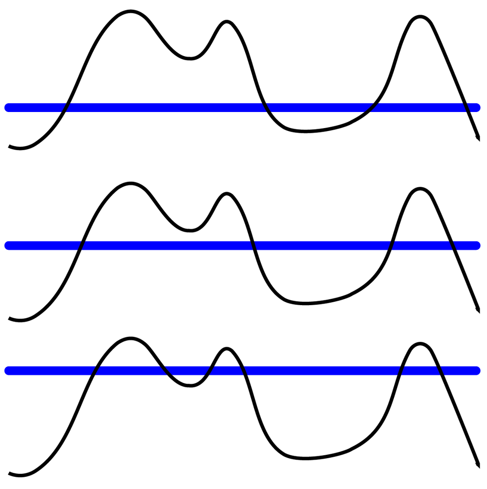
One technique for analyzing networks is called “the island method” (see Figure 4-1); it is particularly well-suited to valued networks such as the Egypt Twitter network that we are using as sample data.
The island method works as follows: imagine our network as an island with a complex terrain, where the height of each point on the terrain is defined by the value of a node (e.g., degree centrality) or edge (e.g., number of retweets). Now let us imagine that the water level around this island is rising slowly, leaving portions of the landscape underwater. When the valleys in the island are flooded, the island essentially splits into smaller islands—revealing where the highest peaks are, and making these peaks smaller. It is possible to raise the water level so high that the entire island will disappear, so this method needs to be applied judiciously to reveal meaningful results.
In terms of networks, this means that the giant component gets split up into smaller components, and areas with the strongest amount of retweeting activity (subcores) become their own components that can be analyzed separately.
The first thing we need to implement for the island method is a function to virtually raise the water level. The function below takes a graph, and applies a threshold (“water level”), letting all edges above a certain value through, and removing all others. Don’t worry—it returns a copy of the original graph, so it’s non-destructive:
def trim_edges(g, weight=1):
        g2=net.Graph()
        for f, to, edata in g.edges(data=True):
                if edata['weight'] > weight:
                        g2.add_edge(f,to,edata)
        return g2
Now, let’s define how the water level should be raised. We will compute evenly spaced thresholds and produce a list of networks at each water level:
def island_method(g, iterations=5):
    weights= [edata['weight'] for f,to,edata in g.edges(data=True)]

    mn=int(min(weights))
    mx=int(max(weights))
    #compute the size of the step, so we get a reasonable step in iterations
    step=int((mx-mn)/iterations)

    return [[threshold, trim_edges(g, threshold)] for threshold in range(mn,mx,step)]
This function will return a list of graph objects, each corresponding to a specific water level.
Now let’s isolate the biggest component of the Egypt Retweet Network, and separate it into subparts using the island method:
>>> cc=net.connected_component_subgraphs(e)[0]
>>> islands=island_method(cc)
>>> for i in islands:
...  # print the threshold level, size of the graph, and number of connected components
...  print i[0], len(i[1]), len(net.connected_component_subgraphs(i[1]))

        1 12360 314
        62 27 11
        123 8 3
        184 5 2
        245 5 2
What does this mean? When all links with a value of 1 (i.e., single retweets) are dropped, the network separates into 314 island subgraphs—each representing a group of people retweeting repeatedly from each other. Since single retweets could be considered accidental, this is a very useful result—repeated retweets are more likely to happen between groups of people that communicate repeatedly and thus have developed some kind of a trust relationship.
Thresholding at the value of 62 (i.e., 62 repeat retweets for each pair of nodes) reveals that there are only 27 nodes left, in 11 islands. In this case, it’s the highest meaningful threshold—the remaining 27 nodes are the people most actively involved in the Tahrir Square protests, and journalists covering the events.
It may take some trial and error, but a well-tuned “water level” can yield a very meaningful analysis of a large network—instantly zeroing in on the cores of the most activity.
Subgraphs—Ego Networks
Ego networks are subnetworks that are centered on a certain node. On Facebook and LinkedIn, these are simply described as “your network”—but you can only access your own ego networks, and can’t do a broader survey. Having a larger dataset allows us to survey and compare ego networks of various people.
We derive ego networks by running a breath-first search (described in Breadth-First Traversal), and limiting the depth of our search (network radius) to a small value, usually not more than 3. While in traditional BFS we build a tree of links we followed to get to a node, to produce an ego network we capture all links between node’s neighbors.
To explain the reasoning behind using a small search depth, we should revisit the idea of what it means to be connected in a social network, and what network distance means. In the most basic case, a link means that “Alice is friends with Bob,” a distance of 2 means “Carol is a friend of a friend of Alice,” and a distance of 3 means that “Dave is a friend of a friend of a friend of Alice.” Intuitively, we understand that while we know quite a bit about our friends, and we know something about some of our friends’ friends, we know nearly nothing about our friends’ friends’ friends.
Formally, this concept is known as a Horizon of Observability,[25] a concept loosely borrowed from physics and the notion of the observable universe. Noah Friedkin observed that in social networks, people had a relatively high degree of knowledge of their own immediate social networks (~30% error rate), which is about as good as self-reported data can be. The error rate jumps to 70% for 2 degrees of separation, and to nearly 100% at 3.
In online networks such as Twitter, with a significantly looser definition of a “friend” and computer-facilitated retention of information, the useful radius of the ego network is much larger. However, trust and influence still travel over the less-reliable “wetware” interpersonal channels, so it would be a mistake to consider ego networks with a radius over 3. Depth-first search may be used instead to determine the penetration of a message via a sequence of retweets—a technique that we will address in Chapter 6.
Extracting and Visualizing Ego Networks with Python
Extraction of ego networks is quite simple—as NetworkX provides a ready-made function to do the job:
>>> net.ego_graph(cc,'justinbieber')
<networkx.classes.multigraph.MultiGraph object at 0x1ad54090>
Yes, believe it or not, Justin Bieber is in the Egypt Retweet dataset. His ego network was shown early on in the book, in Figure 1-11.
The ego_graph function
returns a NetworkX graph object, and all the usual metrics (degree,
betweenness, etc.,) can be computed on it.
However, a couple other simple metrics stand out as well. Knowing the size of an ego network is important to understand the reach of the information that a person can transmit (or, conversely, have access to).
The other metric is called clustering coefficient—essentially, it measures the proportion of your friends that are also friends with each other (i.e., what amount of mutual trust people have for each other). This metric can be applied to entire networks—but in a large network with widely varying densities and multiple cores, average clustering is difficult to interpret. In ego networks, the interpretation is simple—dense ego networks with a lot of mutual trust have a high clustering coefficient. Star networks with a single broadcast node and passive listeners have a low clustering coefficient.
Let us explore a couple ego networks in the Egypt data:
## we need to convert the ego network from a Multi-graph to a simple Graph
>>> bieb = net.Graph(net.ego_graph(cc,'justinbieber', radius=2))
>>> len(bieb)
22
>>> net.average_clustering(bieb)
0.0
The celebrity status of Justin Bieber doesn’t help him in this particular case—of his (at the time) 9 million followers, only 22 have retweeted his messages about the Egyptian uprising. His clustering coefficient shows that he is a pure broadcaster and is not embedded in a trust network of fans—or, at least, he is not in a trust network that cares about world politics.[26]
Let us now explore a celebrity of a different kind—Wael Ghonim, the face of the new generation of Egyptians, a Google executive, and a prolific tweeter:
>>> ghonim= net.Graph(net.ego_graph(cc,'Ghonim', radius=2))
>>> len(ghonim)
3450
>>> net.average_clustering(ghonim)
0.22613518489812276
Not only does Wael Ghonim have a vastly larger retweet network (despite having 100 times fewer followers than Bieber), his ego network is a network of trust where people retweet messages from him and from each other—a network where a revolutionary message can easily spread and be sustained.
The structural hole and triadic analysis that we will discuss in the next section is also very applicable to ego networks—so stay tuned and improvise with your data!
Triads
A triad is simply three nodes interlinked in some way. However, in triad analysis, things are really not so simple. All possible undirected triads are shown in Figure 4-2; as you can see, only the first two have all of their nodes interconnected, and thus present a significant interest. There are 16 possible directed triads, but we shall defer that discussion until a little later in the chapter.
The closed triad (on the left in Figure 4-2) represents a fully connected group: A, B, and C are connected to each other with equivalently strong ties. The most basic example of a triad like this is a “nuclear family”—mother (Alice), father (Bob) and a child (Carol). Of course, these triads can overlap—for example, the same mother and father might have another child (Dan), in which case there is not one triad, but 4:
[alice, bob, carol]
[alice, bob, dave]
[carol, dave, alice]
[carol, dave, bob]
This network structure represents perhaps the oldest piece of research in the entire field. In 1908, Georg Simmel, a contemporary of Max Weber and a member of his intellectual circles, authored a piece called “The Treatise on the Triad”.[27]
He wrote that in a dyad (i.e., two nodes connected to each other), each person is able to retain their individuality while maintaining a close relationship. Exchange of information and ideas happens, but at the same time it does not subjugate the individual to the group. In a triad, the third individual becomes at a source of balance (providing second opinions and calming nerves). However, the third node is also a feedback loop—information from A can pass to B, then to C, and back to A—in a much distorted form, as a childrens’ game of “Telephone” shows.
As a result of accumulating distortions, a triad over time generates a set of artifacts that are private to the triad—local jargon or nicknames, local norms and rules of behavior, shared stories. In a macro-context, sociologists would call an accumulation of these artifacts, culture.
Perhaps in a context of one triad, this is a very big word to use—but think of your own family or the families of your friends. Or, download an episode of ABC’s “Wife Swap” reality show (mercifully cancelled in 2009) and watch cultures of two families collide on reality TV.[28]
Fraternity Study—Tie Stability and Triads
Another study in the same milieu was done by Newcomb. [29] In fact, this study is somewhat (disturbingly) similar to modern reality TV, but was conducted in the early 1960s. Imagine a fraternity in Michigan (yes, there was beer). At the beginning of a semester, 17 students (all white men) were recruited to live in a frat house for a semester, in exchange for their personal data. Every week, researchers interviewed every one of the students asking them to rank their interactions with their fraternity brothers from 1 (best) to 16 (worst).
The findings of this study were that:
Asymmetric ties (e.g., “I like you more than you like me”) were the least stable of all, lasting no more than two weeks.
Symmetric ties (dyads where 2 people like each other about equally) were significantly more stable.
Triadic structures were the most stable over time, with students smoothing over conflicts, organizing events (parties?) together, and overall defining the tone of interaction among the fraternity brothers.
Triads and Terrorists
In the beginning of the book (Informal Networks in Terrorist Cells), we mentioned that Al Qaeda cells were often sequestered in safe-houses during training and preparation for terrorist attacks. This sequestration forced the cells to form a dense triadic structure, with everyone embedded in triads with everyone else. Combined with a virtual sensory deprivation (all information from the outside world arrived highly filtered through the cell leader), the groups generate their own cultural artifacts that go beyond nicknames and shared stories—but rather continue to define their identity as religious extremist and reinforcing their resolve to complete the attack.
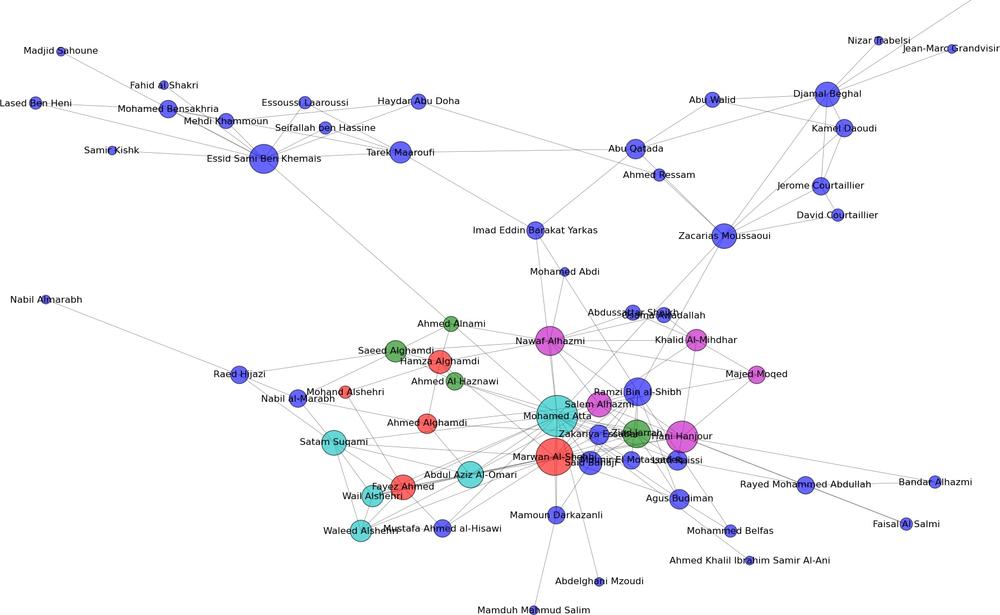
The Hamburg Cell (which started the planning for 9/11 and ultimately participated in the attack) was—to quote Mark Sageman,[30] “just a bunch of guys.” After studying the lives of 172 terrorists, Sageman found the most common factor driving them was the social ties within their cell. Most started as friends, colleagues, or relatives—and were drawn closer by bonds of friendship, loyalty, solidarity and trust, and rewarded by a powerful sense of belonging and collective identity.
In the book’s GitHub repository (https://github.com/maksim2042/SNABook/chapter4), you can find the data used to generate the picture in Figure 4-3 [31] and analyze it yourself. The data is supplied in an edge-list file, in a format resembling the following:
Hani Hanjour,Majed Moqed,5,1
Hani Hanjour,Nawaf Alhazmi,5,1
Hani Hanjour,Khalid Al-Mihdhar,5,1
The first column is the name of the “from” node, the second column is the name of the “to” node, and the following two numbers signify the strength of tie (5=strong tie, 1=weak tie); and the level to which the tie has been verified (1 = confirmed close contact, 2 = various recorded interactions, 3 = potential or planned or unconfirmed interactions).
To read this file, we will not be able to use NetworkX’s built-in file readers, but we can build one in just a few lines of code:
import csv ## we'll use the built-in CSV library
import networkx as net

# open the file
in_file=csv.reader(open('9_11_edgelist.txt','rb'))

g=net.Graph()
for line in in_file:
    g.add_edge(line[0],line[1],weight=line[2],conf=line[3])
We also have an attribute file that marks the 19 hijackers by the flight that they were on. Let’s read this file as well:
#first, let's make sure that all nodes in the graph have the 'flight' attribute
for n in g.nodes_iter(): g.node[n]['flight']='None'

attrb=csv.reader(open('9_11_attrib.txt','rb'))
for line in attrb:
    g.node[line[0]]['flight']=line[1]
Note
There are two ways to list nodes in the graph. g.nodes() produces a list of nodes, and
g.nodes_iter() produces a Python
iterator. An iterator is limited to use in
loops only—but takes significantly less memory and is faster on
large graphs.
If you plotted the network right now using the default net.draw(g) function, you would find that
the network consists of several disconnected components. This is due
to the data being largely fragmentary and incomplete; we should
concern ourselves with the largest component of the network
only:
# Connected_component_subgraphs() returns a list of components,
# sorted largest to smallest
components=net.connected_component_subgraphs(g)

# pick the first and largest component
cc = components[0]
We use a custom plotting function in multimode.py to plot the picture. The function reads node attributes and assigns colors to them based on attribute values, creating a custom color-map on the fly:
import networkx as net
import matplotlib.pyplot as plot
from collections import defaultdict

def plot_multimode(m,layout=net.spring_layout, type_string='type',filename_prefix='',output_type='pdf'):

    ## create a default color order and an empty color-map
    colors=['r','g','b','c','m','y','k']
    colormap={}
    d=net.degree(m)  #we use degree for sizing nodes
    pos=layout(m)  #compute layout

    #Now we need to find groups of nodes that need to be colored differently
    nodesets=defaultdict(list)
    for n in m.nodes():
        t=m.node[n][type_string]
        nodesets[t].append(n)

    ## Draw each group of nodes separately, using its own color settings
    print "drawing nodes..."
    i=0
    for key in nodesets.keys():
        ns=[d[n]*100 for n in nodesets[key]]
        net.draw_networkx_nodes(m,pos,nodelist=nodesets[key], node_size=ns,
                                node_color=colors[i], alpha=0.6)
        colormap[key]=colors[i]
        i+=1
        if i==len(colors):
            i=0  ### wrap around the colormap if we run out of colors
    print colormap

    ## Draw edges using a default drawing mechanism
    print "drawing edges..."
    net.draw_networkx_edges(m,pos,width=0.5,alpha=0.5)
    net.draw_networkx_labels(m,pos,font_size=8)
    plot.axis('off')
    if filename_prefix is not '':
        plot.savefig(filename_prefix+'.'+output_type)
Finally, we plot the networks:
import multimode as mm

# type-string tells the function what attribute to differentiate on
mm.plot_multimode(cc,type_string='flight')
Once we establish the tools for triadic analysis, you can use this data as a test-bed to understand the way triads work, and also potentially link up to the rich literature on terrorism studies.
The “Forbidden Triad” and Structural Holes
My friend Bob[32] has a problem. You see, he is in love with two women. One is a spirited beauty from Eastern Europe (let’s call her Alice), and the other a happy-go-lucky girl from South America named Carolina. Either of the two would have made an excellent match for Bob, but yet he can’t decide. When Bob is with Alice, he longs for Carolina and her lighthearted attitude, and when he’s with Carolina he longs for Alice and her beauty and deep conversations. As a result, after all these years, Bob is still pathologically single.
In terms of networks, Bob’s predicament looks like the second triad in Figure 4-2. B is linked to A, and to C—but A is not in any way linked to C, and should stay that way if Bob wants to keep up the ruse. Every day, this is adding more and more stress to Bob’s life as he needs to coordinate his schedule to make sure A and C never meet, but also needs to make sure that he doesn’t “spill the beans” by failing to remember what he told A or C—or by accidentally passing information from A to C. As a result, Bob is ridden with angst, and the whole thing is really not working out in his favor.
My other friend, a Banker, has a very similar situation in terms of network connections, but in fact is rather happy about it. His A stands for AmeriCorp, Inc and C for CorpAmerica, Inc. AmeriCorp, Inc. deposits money in his bank, expecting an interest payments of 5%. CorpAmerica, Inc. takes out loans, paying an interest rate of 7%. B gets to keep the spread in interest rates—the 2% difference between what C pays and what A expects in interest. In case of my friend, this 2% spread is big enough to pay for a large house, a late-model BMW, an elite country-club membership, and many other material possessions that he enjoys rather conspicuously. Had A and C ever got together for a friendly game of golf, they could agree on A loaning money to C directly at a rate of 6% and realize that both could benefit by cutting out the middleman. Banker B would be rather upset if that happens.
Despite completely different stories behind the triads, Bob’s and Banker’s interests are exactly the same. They need to make sure that the two ends of their open-triad network never communicate directly—that is, never form a link.
The name for this triad varies depending on who you ask. Some researchers call it “the forbidden triad”—because, like Bob, they think it is related to stress, anxiety, and questionable morals of dating two women at the same time. Others call it a “structural hole” or a “brokerage structure” and relate number of structural holes to a person’s ability to perform as an entrepreneur, a banker, a broker or a real-estate agent.
Ron Burt[33] showed in his studies that businessmen who maintained many structural holes had a significantly higher rate of success in a competitive marketplace. This was predicated on two things—the success of businessmen was based on their ability to exploit and trade on asymmetric information, and the businessmen had to have a high tolerance for stress involved in creating and maintaining “arbitrage opportunities.”
Structural Holes and Boundary Spanning
Structural holes have another important mission—since they can span asymmetric information (as both of my friends exploit), they can also bridge entire communities. Both authors of this book are professionals in the field of social network analysis (Max teaches it, and Alex writes analytic software), and professional musicians. In fact, we met at a rock festival where our respective bands performed.
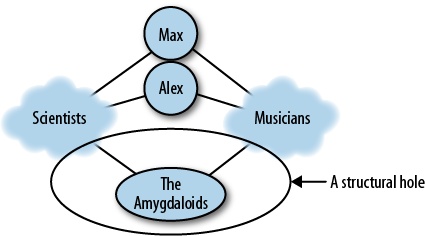
So—a triad that includes Max, Max’s closest collaborator in science, and the drummer in his band is indeed a structural hole. The scientist and the drummer would share some basic understanding of English, but would hardly find enough topics for conversation; a social network tie between them is nearly impossible due to the social distance (a term we will explore further when we discuss information diffusion in Chapter 6).
Our communities (scientists and musicians) intersect more often than one would imagine; Max used to perform with a band that consisted entirely of professors, and a rock band consisting entirely of neuroscientists (called The Amygdaloids) [34] has actually been signed by a label.
However, these boundary spanners (scientist musicians and musician scientists) are still relatively rare compared to the number of people that are only professional musicians or scientists. As a result, the intersection between two communities looks somewhat like Figure 4-4.
In fact, this sort of thing happens on many levels. If we drilled into the “Scientists” cloud, we would find that it consists of major fields (biology, computer science, humanities, etc), and if we drill down further we find that fields consist of subfields, all linked by structural holes.
In the scientific community, this is especially important since many new discoveries are interdisciplinary in nature. For example, James Fowler[35] works at the intersection of social network analysis and neuroscience.
Some other fields (economics is one) discourage communication and cross-publication between subfields, and are very protective of their theories. In these cases, a structural hole position between, say, Austrian and neo-classical economics would be very stressful to sustain—more like Bob’s predicament than that of the Banker.
Triads in Politics
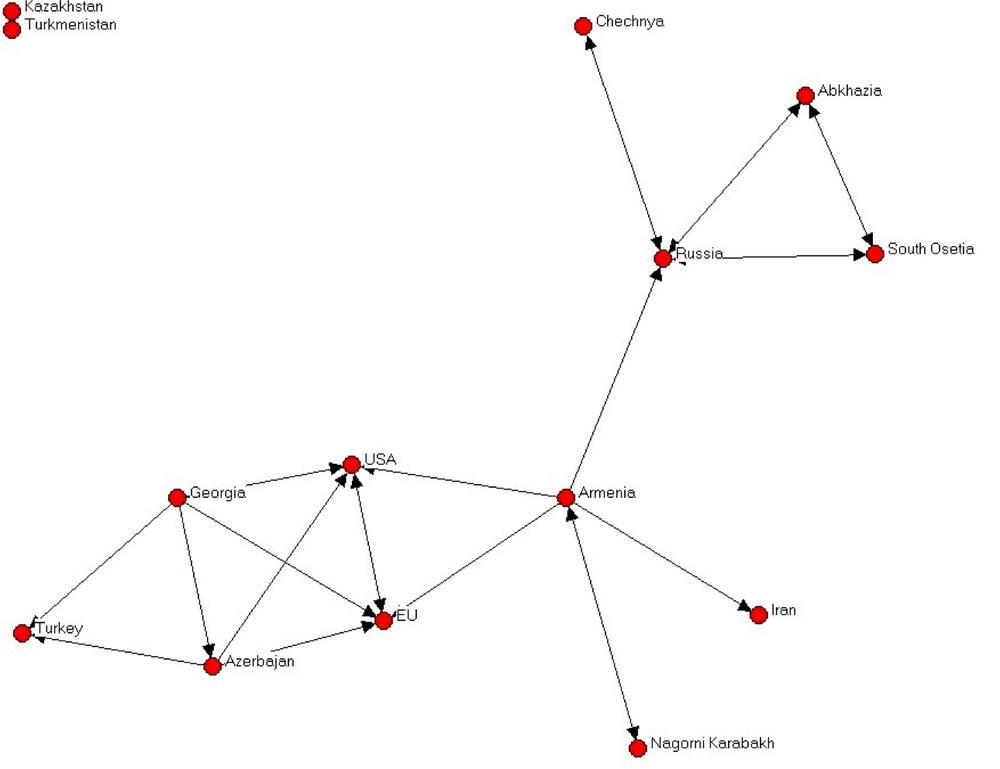
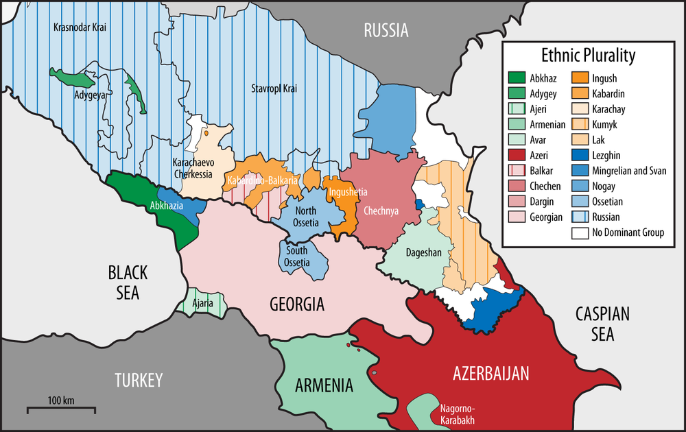
Figure 4-5 shows a network of political cooperation among the countries in the Caucasus. [36] The Caucasus is a very interesting place in terms of modern geopolitics (see the map in Figure 4-6). It’s a fairly small patch of uniquely beautiful mountainous landscape that is sandwiched between Russia on the north, and Turkey and Iran to the south. Its population is a tumultuous mix of Christian and Muslim nations, and their shifting allegiances to the West, Russia, or Turkey have (starting with the disintegration of Soviet Union) created a geopolitical landscape that is full of surprises (mostly unpleasant ones, at least for the local population).
The network in the figure is built by looking at the joint political statements and agreements made by the countries and republics of the Caucasus, Russia, Turkey, EU, and the United States, and clearly shows the different governing styles of Russia and the West. The Russia-centric side of the network shows a system rich in structural holes. Russia is truly in charge, and lateral ties between peripheral actors are almost non-existent.
The single lateral tie is between South Ossetia and Abkhazia. At the time of this study, both of these areas were still technically a part of Georgia—but the fact that they had no allegiance to Georgia was quite apparent at the time. Within two years, South Ossetia became the site of a short but bloody attempt by the Georgian army to squash the separatist movement (alternatively, this was a Russian provocation to cement its influence in the region, depending on whether one listens to Russian or American news sources). Shortly thereafter, both South Ossetia and Abkhazia declared their independence and allied themselves formally with Russia.
Meanwhile, the Western end of the network shows a pattern of closure and multilateral ties. This may be less conducive to influence from the superpowers, as lateral ties reduce efficiency of direct influence. However, at the same time the triadic structures are more stable and require less force to maintain.
Directed Triads
But enough theory, let’s write some code!
Figure 4-7 shows all possible directed triads. In a directed triad, we consider edges that are both one-way and bidirectional; thus instead of 4 possible triads we have 16 variations. We will turn to interpretation of these shapes in a bit, but first let us define a way to catalogue them. This method of counting and cataloguing triads is somewhat arcane, but is a standard for the academic literature in the field and dates back to 1972.[37]
The triads are numbered 1-16, and have a code associated with them. The code reads like this:
The first number is the number of bidirectional edges.
The second number is the number of single edges.
The third number is the number of “non-existent” edges.
A letter code to distinguish directed variations of the same triad—U for “up,” D for “down,” C for “circle,” and T for “transitive” (i.e., having 2 paths that lead to the same endpoint).
Triads 1-3 in the figure are unconnected, triads 4-8 and 11 represent variations on structural holes, and triads 9,10 and 12-16 are variations on closed triads.
Analyzing Triads in Real Networks
The process of triadic analysis in a real network is called the triad census. In this process, for every node we count occurrences of the 16 types of triads to determine the node’s role in the network structure. For example, a node with many occurrences of triads 4, 7, and 11 (i.e., rich in outgoing links and structural holes) is a source of information or possibly a group leader.
To run the triad census, we will need an algorithm that is not included in the NetworkX—the triadic census algorithm.[38] Download the Chapter4 package from GitHub,[39] change the directory to the location of downloaded files, and start Python:
>>> import networkx as net
>>> import tradic
>>> import draw_triads
The draw_triads command will
reproduce Figure 4-7.
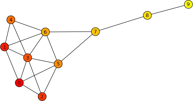
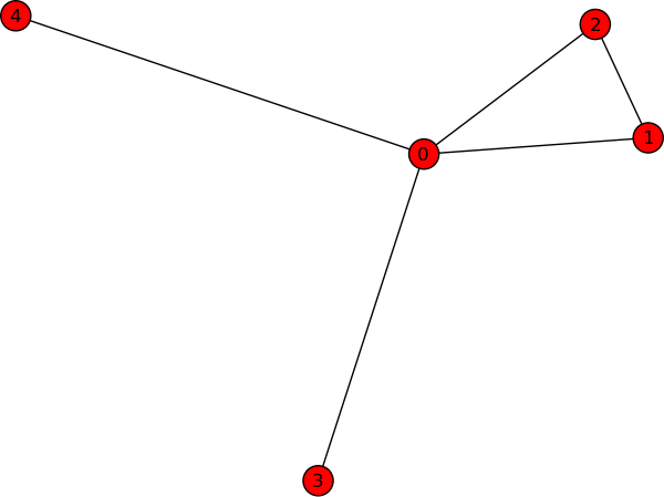
Now, let us apply the triadic census to some sample data (specifically to the kite network in Figure 4-8):
## generate a directed version of the classic "Kite Graph"
>>> g=net.DiGraph(net.krackhardt_kite_graph())

## Run the triadic census
>>> census, node_census = triadic.triadic_census(g)
>>> census
{'201': 24, '021C': 0, '021D': 0, '210': 0,
'120U': 0, '030C': 0, '003': 22, '300': 11,
'012': 0, '021U': 0, '120D': 0, '102': 63,
'111U': 0, '030T': 0, '120C': 0, '111D': 0}
The triadic census function returns two results—a Python dict with overall results for the network, and a dict-of-dicts containing the same results for individual nodes.
In the kite graph, the procedure has counted 24 structural-hole triads (code 201), and 11 closed triads (code 300). What this means is that there are areas of high closure within the network, and areas with many structural holes. Which, of course, is apparent from the sample picture—but may not be so apparent for larger networks.
The ratio between structural hole and closed triads is also important—a hierarchy is largely composed of structural holes, while more egalitarian structures would have a higher ratio of closed triads.
In short, a triadic census lets one make high-level conclusions about the network structure in a macro form. However, the micro form is more interesting. The code below generates a triadic census table, and its results are in Table 4-1:
keys=node_census.values()[1].keys()

## Generate a table header
print '| Node |', ' | '.join(keys)

## Generate table contents
## A little magic is required to convert ints to strings
for k in node_census.keys():
  print '|', k, '|',' | '.join([str(v) for v in node_census[k].values()])
| Node | 201 | 021C | 021D | 210 | 120U | 030C | 003 | 300 | 012 | 021U | 120D | 102 | 111U | 030T | 120C | 111D |
0 | 8 | 0 | 0 | 0 | 0 | 0 | 0 | 4 | 0 | 0 | 0 | 14 | 0 | 0 | 0 | 0 |
1 | 4 | 0 | 0 | 0 | 0 | 0 | 0 | 3 | 0 | 0 | 0 | 11 | 0 | 0 | 0 | 0 |
2 | 4 | 0 | 0 | 0 | 0 | 0 | 0 | 1 | 0 | 0 | 0 | 7 | 0 | 0 | 0 | 0 |
3 | 3 | 0 | 0 | 0 | 0 | 0 | 0 | 2 | 0 | 0 | 0 | 7 | 0 | 0 | 0 | 0 |
4 | 2 | 0 | 0 | 0 | 0 | 0 | 0 | 0 | 0 | 0 | 0 | 4 | 0 | 0 | 0 | 0 |
5 | 1 | 0 | 0 | 0 | 0 | 0 | 0 | 1 | 0 | 0 | 0 | 5 | 0 | 0 | 0 | 0 |
6 | 1 | 0 | 0 | 0 | 0 | 0 | 0 | 0 | 0 | 0 | 0 | 3 | 0 | 0 | 0 | 0 |
7 | 1 | 0 | 0 | 0 | 0 | 0 | 0 | 0 | 0 | 0 | 0 | 5 | 0 | 0 | 0 | 0 |
8 | 0 | 0 | 0 | 0 | 0 | 0 | 0 | 0 | 0 | 0 | 0 | 7 | 0 | 0 | 0 | 0 |
9 | 0 | 0 | 0 | 0 | 0 | 0 | 0 | 0 | 0 | 0 | 0 | 0 | 0 | 0 | 0 | 0 |
Let’s look at the main types of triads: the closed triad (code 300) and the structural hole triad (code 201).
Real Data
Let’s now run a triadic census on the 9/11 hijackers data we used earlier in the chapter, and find out who had the most cliques (closed triads, or triad 300):
census, node_census = triadic.triadic_census(cc)

## get only the number of closed triads, and sort the list by the value, descending
closed_triads=[[-k,v] for k,v in sorted([[-node_census[k]['300'],k] for k in node_census.keys()])]
The top person in the list has a familiar name: Mohammed Atta was part of the original Hamburg cell that planned the September 11th attacks, and served as the hijacker-pilot of American Airlines Flight 11, crashing the plane into the North Tower of the World Trade Center.
Cliques
While we might have an intuitive understanding of a clique in a social network as a cohesive group of people that are tightly connected to each other (and not tightly connected to people outside the group), in the field of SNA there is a formal mathematical definition that is quite a bit more rigorous.
A clique is defined as a maximal complete subgraph of a given graph—i.e., a group of people where everybody is connected directly to everyone else. The word “maximal” means that no other nodes can be added to the clique without making it less connected. Essentially, a clique consists of several overlapping closed triads, and inherits many of the culture-generating, and amplification properties of closed triads.
A clique must generate consensus or fall apart—which is why in the vernacular, cliques are often viewed in conflict with other cliques. It is, in fact, very easy to agree about conflict, and having a common enemy (or a group of common enemies) helps cliques unite. We will discuss some of the implication of conflict and cliques in Chapter 6.
But for now, let us see if we can locate cliques in some sample networks.
Detecting Cliques
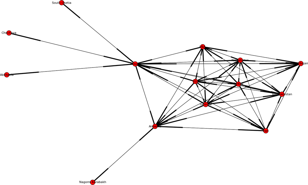
As a test dataset, let us take another look at the data on geopolitics of the Caucasus. This time, we’ll explore economic relations between the countries (Figure 4-9). The dataset rates level of economic cooperation on the scale of 0 to 1—where 1 is a close or exclusive tie, and 0 is the complete lack of economic cooperation:
>>> eco=net.read_pajek("economic.net")
>>> net.draw(eco)The dataset clearly shows that there are two distinct sides to the region—the Western-centric side and the Russia-centric side; local and regional economic ties are frequently non-existent, as the nearest geographical neighbors (e.g., Armenia and Azerbaijan) consider each other to be enemies and structure their relationships with the superpowers accordingly. Iran and Turkey act as “spoilers”—a country with significant economic ties to Iran cannot have ties to the US, and thus is forced to ally itself with Russia. Of course, oil and natural gas interests play a significant role as well.
A structure like this is ripe for development of cliques. Let’s see if we can find them. First, we will drop the low-level connections (< 0.5) to isolate the core:
>>> e2=trim_edges(eco, weight=0.5)
>>> cliques = list(net.find_cliques(eco))
>>> cliques
[['EU', 'Turkey', 'Russia'],
['EU', 'Turkey', 'USA'],
['EU', 'Azerbajan'],
['EU', 'Georgia'],
['EU', 'Kazakhstan', 'Russia'],
['EU', 'Kazakhstan', 'USA'], ['EU', 'Armenia'],
['South Osetia', 'Russia'],
['Nagorni Karabakh', 'Armenia'],
['Chechnya', 'Russia'],
['Abkhazia', 'Russia']]
Let’s walk through the clique output. First,
- [EU, Turkey, Russia], [EU, Turkey, USA]
Represents the superpowers and the two sides of the debate whether Turkey should enter the EU as a member.
- EU, Azerbaijan], [EU, Georgia]
The Western-allied countries in the Caucasus; Azerbaijan is a major oil producer and a BP-owned pipeline crosses from Azerbaijan through Georgia on its way to the Black Sea.
- [South Ossetia, Russia], [Nagorni Karabakh, Armenia], [Chechnya, Russia], [Abkhazia, Russia]
All recent conflicts where allegiances of minor local republics shifted from West to Russia (by will or by force).
- [EU, Kazakhstan, Russia], [EU, Kazakhstan, USA]
Kazakhstan is a major producer of natural gas, which is sold to both EU and the US by means of Russian-owned pipelines and Liquid Natural Gas (LNG) facilities.
In short—the clique algorithm produces an output that can be quickly interpreted by a human who is versed in the field.
Unfortunately, the cliques frequently overlap, and a single event or phenomena might result in multiple cliques. Other algorithms (n-clans, k_plexes, etc) exist to help solve this problem—but they are not yet implemented in NetworkX, and their implementation is beyond the scope of this book.
We will address this problem using clustering methods in the next sections.
Hierarchical Clustering
The next class of algorithms we will touch on—though briefly—is clustering algorithms. The universe of clustering algorithms is large and varied, and perhaps best addressed by other books—but I will briefly touch on the application of clustering algorithms to social network analysis and provide a quick example of useful insights that can be derived from them.
Let’s first start by returning to the notion of distance. We can define distance in many ways—from geographical distance to ground travel distance to time-based distance (i.e., how long it takes to get from point A to point B), and so on. In social networks, we find two types of distance most useful; a graph distance (or path length) between pairs of nodes, and a similarity-based distance (that is, we consider nodes to be closer together if they are similar in some way).
In the Caucasus network that we used in the previous section, the graph distance matrix looks like Table 4-2.
| TR | SO | GE | IR | TK | US | AZ | CH | AR | EU | NK | KZ | RU | AB | |
TR | 0 | 2 | 1 | 1 | 1 | 1 | 1 | 2 | 1 | 1 | 2 | 1 | 1 | 2 |
SO | 2 | 0 | 2 | 2 | 2 | 2 | 2 | 2 | 2 | 2 | 3 | 2 | 1 | 2 |
GE | 1 | 2 | 0 | 1 | 1 | 1 | 1 | 2 | 1 | 1 | 2 | 1 | 1 | 2 |
IR | 1 | 2 | 1 | 0 | 1 | 2 | 1 | 2 | 1 | 1 | 2 | 1 | 1 | 2 |
TK | 1 | 2 | 1 | 1 | 0 | 1 | 1 | 2 | 1 | 1 | 2 | 1 | 1 | 0 |
US | 1 | 2 | 1 | 2 | 1 | 0 | 1 | 2 | 1 | 1 | 2 | 1 | 1 | 2 |
AZ | 1 | 2 | 1 | 1 | 1 | 1 | 0 | 2 | 2 | 1 | 3 | 1 | 1 | 3 |
CH | 2 | 2 | 2 | 2 | 2 | 2 | 2 | 0 | 2 | 2 | 3 | 2 | 1 | 2 |
AR | 1 | 2 | 1 | 1 | 1 | 1 | 2 | 2 | 0 | 1 | 1 | 1 | 1 | 2 |
EU | 1 | 2 | 1 | 1 | 1 | 1 | 1 | 2 | 1 | 0 | 2 | 1 | 1 | 2 |
NK | 2 | 3 | 2 | 2 | 2 | 2 | 3 | 3 | 1 | 2 | 0 | 2 | 2 | 2 |
KZ | 1 | 2 | 1 | 1 | 1 | 1 | 1 | 2 | 1 | 1 | 2 | 0 | 1 | 2 |
RU | 1 | 1 | 1 | 1 | 1 | 1 | 1 | 1 | 1 | 1 | 2 | 1 | 0 | 1 |
AB | 2 | 2 | 2 | 2 | 0 | 2 | 3 | 2 | 2 | 2 | 2 | 2 | 1 | 0 |
This, of course, is quite different from the geographic distances—and illustrates the fact that allegiances in the region are interleaved, with every one of the actors surrounded not by local allies, but by potential adversaries.
Let us now see if we can find the adversarial clusters in the economic network. We will use a hierarchical clustering routine in SciPy, and a snippet of code originally written by Drew Conway[40] but modified extensively for this book.
The Algorithm
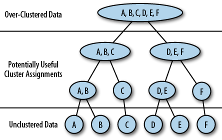
Figure 4-10 shows (in a stylized way) the hierarchical clustering algorithm. The algorithm works roughly as follows:
Starting at the lowest level, every node is assigned its own cluster.
Using the distance table (Table 4-2), find the closest pair of nodes and merge them into a cluster
Recompute the distance table, treating the newly merged cluster as a new node.
Repeat steps 2 and 3, until all nodes in the network have been merged into a single large cluster (top level of the diagram).
Choose a useful clustering threshold between the bottom and top levels—this still requires an intervention from a human analyst and can’t be automated.
Step 3 merits further consideration. How does one go about computing the distance between a cluster a node, or between two clusters? There are three common methods for doing this:
Single-link: merge two clusters with the smallest minimum pairwise distance
Average-link: merge two clusters with the smallest average pairwise distance
Maximum-link or Complete-link: merge the two clusters with the smallest maximum pairwise distance
The complete-link method is considered most sensitive to outliers, and the single-link method tends to form long chains of clusters that may not correspond to our intuitive understanding of what the clusters mean. Average-link method is considered a compromise between the two, and is in fact the most frequently used.
Clustering Cities
To better demonstrate how clustering work, let us consider a sample problem of clustering cities in the Continental U.S. The initial distance table is below; we will use single-link clustering:
| BOS | NY | DC | MIA | CHI | SEA | SF | LA | DEN | |
BOS | 0 | 206 | 429 | 1504 | 963 | 2976 | 3095 | 2979 | 1949 |
NY | 206 | 0 | 233 | 1308 | 802 | 2815 | 2934 | 2786 | 1771 |
DC | 429 | 233 | 0 | 1075 | 671 | 2684 | 2799 | 2631 | 1616 |
MIA | 1504 | 1308 | 1075 | 0 | 1329 | 3273 | 3053 | 2687 | 2037 |
CHI | 963 | 802 | 671 | 1329 | 0 | 2013 | 2142 | 2054 | 996 |
SEA | 2976 | 2815 | 2684 | 3273 | 2013 | 0 | 808 | 1131 | 1307 |
SF | 3095 | 2934 | 2799 | 3053 | 2142 | 808 | 0 | 379 | 1235 |
LA | 2979 | 2786 | 2631 | 2687 | 2054 | 1131 | 379 | 0 | 1059 |
DEN | 1949 | 1771 | 1616 | 2037 | 996 | 1307 | 1235 | 1059 | 0 |
In the first two steps, we will merge Boston, New York, and Washington, DC into a single cluster. Already, we see that the East Coast is emerging as a cluster of its own:
| BS/NY/DC | MIA | CHI | SEA | SF | LA | DEN | |
BS/NY/DC | 0 | 1075 | 671 | 2684 | 2799 | 2631 | 1616 |
MIA | 1075 | 0 | 1329 | 3273 | 3053 | 2687 | 2037 |
CHI | 671 | 1329 | 0 | 2013 | 2142 | 2054 | 996 |
SEA | 2684 | 3273 | 2013 | 0 | 808 | 1131 | 1307 |
SF | 2799 | 3053 | 2142 | 808 | 0 | 379 | 1235 |
LA | 2631 | 2687 | 2054 | 1131 | 379 | 0 | 1059 |
DEN | 1616 | 2037 | 996 | 1307 | 1235 | 1059 | 0 |
Skipping a few more steps, Chicago joins the East Coast cluster, and San Francisco, LA, and Seattle form the West Coast cluster. Technically, Chicago and Denver should form a Midwest cluster—but since we are using the single-link distance metric, Chicago ends up being closer to the East Coast cluster than it is to Denver.
| BOS/NY/DC/CHI | MIA | SF/LA/SEA | DEN | |
BOS/NY/DC/CHI | 0 | 1075 | 2013 | 996 |
MIA | 1075 | 0 | 2687 | |
2037 | SF/LA/SEA | 2054 | 2687 | 0 |
1059 | DEN | 996 | 2037 | 1059 |
This only leaves Miami and Denver unassigned. In the next steps, Denver joins Chicago in the East Coast cluster. At this point, I would argue that clustering no longer makes any sense.
The long chain reaching West from the East Coast cluster to Chicago and on to Denver is a well-known shortfall of the single-distance metric. If we were to use average-link metric in the same context, clustering would be cleaner. The tradeoff for cleaner results is a higher computational complexity—making average-link clustering unsuitable for very large datasets.
Preparing Data and Clustering
Let us now apply hierarchical clustering to the Caucasus data. First, the distance matrix needs to be computed. NetworkX provides the function to generate such a matrix—but it is returned as a dict of dicts. This is a format unsuitable for further computation and needs to be moved into a SciPy matrix. Since matrices do not preserve node labels, we construct a separate array to store node labels.
Finally, we run the SciPy hierarchical clustering routines and produce the entire cluster dendrogram, reminiscent of Figure 4-10. We will need to threshold it at a certain number—here it’s picked arbitrarily, but it’s a parameter, so it can be easily tweaked to achieve more meaningful results.
__author__="""\n""".join(['Maksim Tsvetovat <maksim@tsvetovat.org','Drew Conway <drew.conway@nyu.edu>','Aric Hagberg <hagberg@lanl.gov>'])fromcollectionsimportdefaultdictimportnetworkxasnximportnumpyfromscipy.clusterimporthierarchyfromscipy.spatialimportdistanceimportmatplotlib.pyplotaspltdefcreate_hc(G,t=1.0):"""Creates hierarchical cluster of graph G from distance matrixMaksim Tsvetovat ->> Generalized HC pre- and post-processing to work on labelled graphsand return labelled clustersThe threshold value is now parameterized; useful range should be determinedexperimentally with each dataset""""""Modified from code by Drew Conway"""## Create a shortest-path distance matrix, while preserving node labelslabels=G.nodes()path_length=nx.all_pairs_shortest_path_length(G)distances=numpy.zeros((len(G),len(G)))i=0foru,pinpath_length.items():j=0forv,dinp.items():distances[i][j]=ddistances[j][i]=difi==j:distances[i][j]=0j+=1i+=1# Create hierarchical clusterY=distance.squareform(distances)Z=hierarchy.complete(Y)# Creates HC using farthest point linkage# This partition selection is arbitrary, for illustrive purposesmembership=list(hierarchy.fcluster(Z,t=t))# Create collection of lists for blockmodelpartition=defaultdict(list)forn,pinzip(list(range(len(G))),membership):partition[p].append(labels[n])returnlist(partition.values())
To run the hiclus
algorithm:
>>> import hc
>>> hc.create_hc(eco)
[['Turkmenistan', 'Nagorni Karabakh', 'Russia', 'Abkhazia'],
['USA', 'Armenia', 'EU', 'Kazakhstan'],
['Turkey', 'Georgia', 'Iran', 'Azerbaijan'],
['Chechnya'], ['South Osetia']]
The result is intuitively very readable—[Turkmenistan, Nagorni Karabakh, Russia, Abkhazia] is a Russia-centric cluster; the [USA, Armenia, EU, Kazakhstan] cluster makes a lot of sense around natural gas sale and transport; and the [Turkey, Georgia, Iran, Azerbaijan] cluster reflects pro-Islamic and pro-Persian attitudes. Georgia is somewhat of a misfit because it is Christian and Western-allied politically—but its economic ties to Azerbaijan and Turkey are crucial and thus overshadow its Western outlook. The reset of the clustering is filled with outliers—actually, both are small countries that have caused the world quite a bit of trouble.
Block Models
A block model is a simplified network derived from the original network, where all nodes in a cluster are considered a single node, and all relationships between original nodes become aggregated into relationships between blocks.
In our sample data, a block model shows relationships between the Russia-centric, Western-oriented, and Islamic-oriented clusters (0, 1, and 2). Clusters 3 and 4 are small republics that have significant ties with Russia, but almost no ties with anyone else—due to the highly centralized nature of Russia’s management of its subsidiaries.
To compute the block model, first compute and save a hierarchical clustering, then run the block model on the original graph and supply the clusters as a list of partitions. This should look something like Figure 4-11:
>>> clusters=hc.create_hc(eco)
>>> M=nx.blockmodel(eco,clusters)
>>> net.draw(M)
A slightly more involved drawing mechanism that works on all graphs can be found in hiclus_blockmodel.py:
__author__="""\n""".join(['Maksim Tsvetovat <maksim@tsvetovat.org','Drew Conway <drew.conway@nyu.edu>','Aric Hagberg <hagberg@lanl.gov>'])fromcollectionsimportdefaultdictimportnetworkxasnximportnumpyfromscipy.clusterimporthierarchyfromscipy.spatialimportdistanceimportmatplotlib.pyplotaspltimporthc"""Draw a blockmodel diagram of a clustering alongside the original network"""defhiclus_blockmodel(G):# Extract largest connected component into graph HH=nx.connected_component_subgraphs(G)[0]# Create parititions with hierarchical clusteringpartitions=hc.create_hc(H)# Build blockmodel graphBM=nx.blockmodel(H,partitions)# Draw original graphpos=nx.spring_layout(H,iterations=100)fig=plt.figure(1,figsize=(6,10))ax=fig.add_subplot(211)nx.draw(H,pos,with_labels=False,node_size=10)plt.xlim(0,1)plt.ylim(0,1)# Draw block model with weighted edges and nodes sized by# number of internal nodesnode_size=[BM.node[x]['nnodes']*10forxinBM.nodes()]edge_width=[(2*d['weight'])for(u,v,d)inBM.edges(data=True)]# Set positions to mean of positions of internal nodes from original graphposBM={}forninBM:xy=numpy.array([pos[u]foruinBM.node[n]['graph']])posBM[n]=xy.mean(axis=0)ax=fig.add_subplot(212)nx.draw(BM,posBM,node_size=node_size,width=edge_width,with_labels=False)plt.xlim(0,1)plt.ylim(0,1)plt.axis('off')
Triads, Network Density, and Conflict
In this chapter—actually, for all of the book so far—we have talked about uniform networks that contain one type of node, and one type of edge. However, things are about to get more interesting.
Let us suppose that instead of a single link type we now have two—friendship and conflict. We will also introduce some dynamics, on both the dyadic and triadic level.
We have all witnessed social turmoil—or even have been involved in the midst of it. A long-married couple decides to divorce, and suddenly their friends are faced with difficult decisions. They may feel pressured to side with one partner or the other, potentially splitting long-standing friendships and dividing a formerly cohesive network into “his side” and “her side.” As the wounds of the split-up heal, the space is opened up for creation of new friendships and romantic relationships, and the cycle starts again.
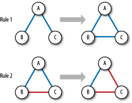
We can model this process using a few very simple rules:
Friend of my friend is my friend (close a structural hole)
Enemy of my friend is my enemy (achieve a balanced triad)
Friend of my enemy is my enemy
Enemy of my enemy is my friend
Actually, rules 2,3, and 4 all describe the same (undirected) triad, just from a different point of view; we’ll call them all “Rule 2” (Figure 4-12). These rules are, in fact, some of the first attempts to describe social complexity in the history of civilization; the first written mention of these rules is in the Bible (Exodus 23:22, with a number of other mentions).
Let’s start with the behavior of a social network without either Rule 1 or Rule 2: if we start with a set of unconnected nodes and connect them randomly at a constant, we will at the end receive a simple random graph with a normal distribution of node degrees (an Erdos random graph). The density of the network (i.e., the number of connections vs. number of possible connections) will rise until every node is connected to every other node (a complete graph or a clique). This, of course, is not terribly interesting.
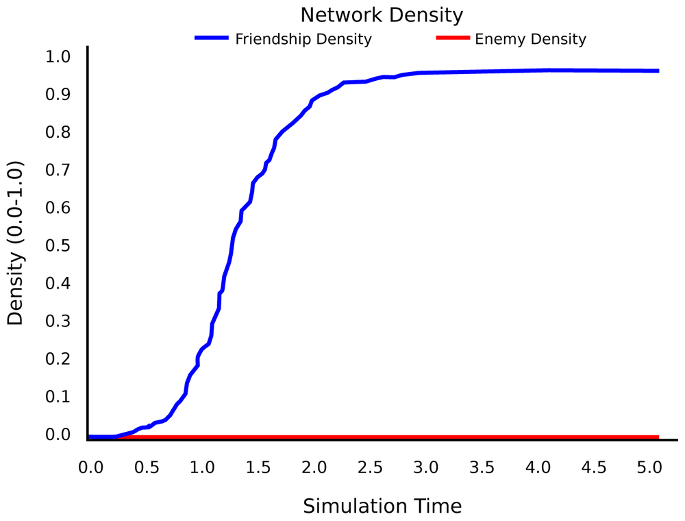
Let us now turn on Rule 1. If an open triad A→B→C is detected, with some probability we will also add a link A→ C. We are still adding links randomly, so at first, the network will grow linearly. At a certain point, a critical mass of connection has been created, and every new connection is likely to create an open triad. This open triad is then closed by Rule 1, which may in turn create more open triads, which then get closed, and so on.
In a sense, the network passes from a linear growth to an exponential growth. It goes viral! (Figure 4-13) The density of connections increases rapidly, until no new connections can be made and we have a complete graph. Of course, in reality, there is a limit to the number of possible connections in the network, a saturation density. This density can be a property of the network itself, or the environment in which the network is developing—or a result of Rule 2 (as in our system).
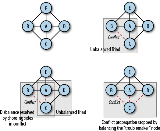
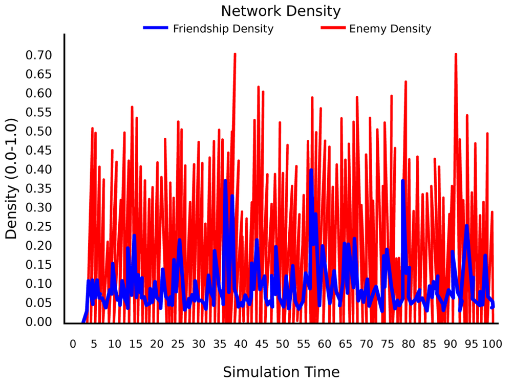
Conflict is introduced in the network at a constant probability, by changing a single friendship tie into an enemy tie. What happens then is illustrated in Figure 4-14. In this simple example, a network consisting of 4 closed triads is struck by a conflict on a single edge. Triad A−B−C becomes unbalanced due to a conflict between B and C; thus A is forced to take sides in the conflict by choosing to remain friends with either B or C, at random. Adding conflict to the A−C edge forces another triad (A−C−D) to become unbalanced, thus drawing agent D into the conflict. If agent D then chooses to isolate C from the rest of the network, the propagation of the conflict can be stopped. However, if instead it separates from A, this will cause the conflict to propagate further and destroy more links. Having more ties increases an agent’s probability of forming even more ties, but also increases the probability that a conflict between two agents will spread throughout the network (Figure 4-14).
As a result, network density no longer grows to near 100%; but instead, once it reaches a second critical mass value, conflicts become more prominent (as can be seen in Figure 4-15) and bring the network density back down. This kind of behavior is called self-organized criticality—my model provides just a simple way to generate such effects in social networks. This is in a way similar to forest fires: the denser the forest, the more likely it is that the next fire will be catastrophic—permitting smaller fires down-regulates the density of the forest to a level where most fires are relatively well-contained.
We will talk more about dynamics of social networks in Chapter 6—but, meanwhile, it is time to start looking at social network data with many different types of nodes—data that can better approximate what we know about social networks.
[25] Friedkin, Noah. “Horizons of Observability and Limits of Informal Control in Organizations.” Social Forces 1983.
[26] This is a sad commentary upon American youth.
[27] A modern translation and commentary can be found in:
Nooteboom, Bart. “Simmel’s Treatise on the Triad (1908)”. Journal of Institutional Economics 2(2006) 365-383.
[28] The authors are not responsible for ensuing brain damage.
[29] Newcomb T. The acquaintance process. New York: Holt, Reinhard & Winston, 1961.
[30] Sageman, Marc. Understanding Terror Networks. University of Pennsylvania Press, 2004.
[31] The original dataset was provided by Valdis Krebs.
[32] Names have been changed to protect the guilty, but the stories are real, if somewhat stylized.
[33] Burt, Ronald. Structural Holes: The Structure of Competition. Cambridge, MA: Harvard University Press, 1992.
[34] www.amygdaloids.com
[35] At the University of California, San Diego (http://jhfowler.ucsd.edu/)
[36] This data comes from a project I did in 2006 in collaboration with the Southern Federal University of Russia.
[37] Davis, J.A. and S. Leinhardt. “The Structure of Positive Interpersonal Relations in Small Groups.” In Sociological Theories in Progress, volume 2, ed. J. Berger. Boston: Houghton Mifflin, 1972.
[38] This algorithm was written by Alex Levenson and Diederik van Liere and submitted to the NetworkX source tree; it may be included in the next release.
Get Social Network Analysis for Startups now with the O’Reilly learning platform.
O’Reilly members experience books, live events, courses curated by job role, and more from O’Reilly and nearly 200 top publishers.
