Tableau Prep: Up & Running

Chapter 4. Shaping Data

As discussed in the previous chapter, the first step of data preparation is understanding how the original data set is structured, followed by determining what structure the data set needs to be in—that is, the desired state—for analysis. This chapter looks at these factors and Prep Builder’s functionality for reshaping data to help you quickly identify how to shape future data sets for analysis.

What to Look for in Incoming Data Sets

Let’s look at a typical input data set from Excel by building a pivot table (Figure 4-1). This example uses sales of ice cream-scented soap.

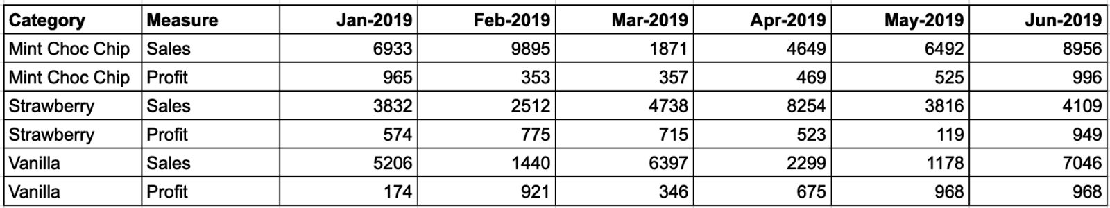
Figure 4-1. Ice Cream Scents sales and profit data

When assessing an incoming data set, it’s important to identify both the dimensions (or categorical values) of the data and the measures. Dimensions is the term Tableau Desktop uses to refer to the columns of data that describe the records example, the regions a product is sold, in or the category that product belongs to). Measures refers to the numeric values of the data set that are being analyzed (such as the number of students in a college class or the tuition they are paying). If the dimensions are all in individual columns, you can move on to measures without having to think about any structural changes. Likewise, you need to assess the measures to ensure each has a separate column in the data set.

The data set from Figure 4-1 has been colored in Figure 4-2 to highlight the structure:

• First two headers: Header for dimension column

• First column values and monthly data headers: Categorical values

• Second column values: Headers for the measure column

• Everything else: Values for the measures columns

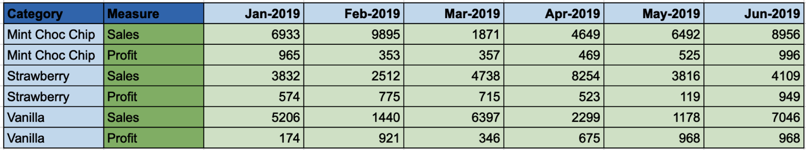
Figure 4-2. Data set broken down into dimensions and measures

By highlighting the structure of the input data set, you can more clearly see what changes you need to make. Once you have this understanding, the process of shaping the data for analysis becomes quicker.

What Shape Is Best for Analysis in Tableau?

When you load data into Tableau Desktop, the software sets the first row of data as the headers for the columns and all subsequent rows as the data points for those headers.¹ Here are the key aspects to consider when structuring data for Desktop:

• Is there a single column for each data field? These columns will form the data fields that are then dragged and dropped in Desktop.

• Is the data field a dimension or measure? Desktop will divide all data fields into dimensions (category) and measures (the numerical values to analyze).

• Is there a single data type for each data field? A data field in Tableau (and most other tools) requires a single data type. Measures must be either an integer or float data type for analysis.

There are a few aspects that do not matter:

Order of columns

Tableau Desktop, Server, and Online will import a data set and order the fields shown in the Data grid in alphabetical order. Therefore, there is no need to order the columns.

Order of the rows

You will analyze the rows through the visualizations you build. The charts and graphs can be sorted, but the rows of data won’t be shown in the order they are imported into the tool, so you don’t need to worry about their order in the data source you are building.²

Geographic roles

These are string fields you assign to location-based fields. Tableau Desktop commonly associates the role you apply (e.g., City or Country) to a longitude and latitude value. In Prep, however, spatial objects (aka shapes) can’t be prescribed for use in Desktop, as the output doesn’t maintain this metadata. The spatial role is often a string data type so that the data field can then be assigned a geographic role in Desktop. The data fields that you wish to assign geographic roles should be cleaned, but no further actions need to be taken. If your data set already contains longitude and latitude values, I recommend you use these, as they are likely to be more detailed than the longitude and latitude values Desktop associates with a geographical role.

Let’s apply these factors to our ice cream scents example in Figure 3-2. We can see the Category column is in the correct state. The Category header is at the top of the column containing all the relevant dimension values.

The Measure header is in the correct location, but is it necessary? The measures are listed under each individual month. One column containing all of the different dates would be more preferable and easier to use to analyze data over time in Tableau. Therefore, in this case, the dates currently listed as headers will need to be pivoted.

The measures that are named in the Measure column would be much easier to analyze if they were individual columns. That would allow us to more simply create totals or averages within either Prep Builder or Tableau Desktop. Having one column labeled Sales and one labeled Profit would enable us to use these two columns as measures when analyzing the data in Desktop.

Now that we’ve identified how we need to shape the data, let’s look at the steps for actually making these changes.

Changing Data Set Structures in Prep Builder

There are four key steps to changing the structure of the input data sets.

Pivot

The Pivot step is the most important one for changing the data structure. There are two types of pivot, as shown in Figure 4-3.

Figure 4-3. Columns-to-rows pivot (Pivot 1) and rows-to-columns pivot (Pivot 2)

Pivot 1, Columns to rows

Converting from multiple columns of data to additional rows of data. The column header is converted into a new dimensional column that will contain all other column headers that are involved in the pivot (Figure 4-4).

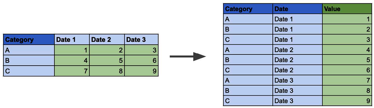
Figure 4-4. The columns-to-rows pivot

Pivot 2, Rows to columns

This is the reverse of the columns-to-rows pivot. In this pivot, rows of data are converted into additional columns within the data set (Figure 4-5). This requires you to select both the column that will become the headers of the new data fields, as well as the data field that will act as the values for the new data fields. If multiple values are forced into the same cell, you’ll need to choose and apply a form of aggregation to them.

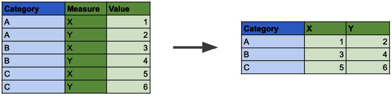
Figure 4-5. The rows-to-columns pivot

Note

Pivots are covered in more detail in Chapters 13 and 14.

Aggregate

The Aggregate step is where values are summed or averaged (Figure 4-6). Aggregations change not only the number of rows, but also potentially the structure of the data.

Figure 4-6. Aggregation icon

The only data fields that continue on in the data flow from this step are those included as a Group By field or an aggregation. In this example, Category is the field we are grouping by and whose values are summed (Figure 4-7).

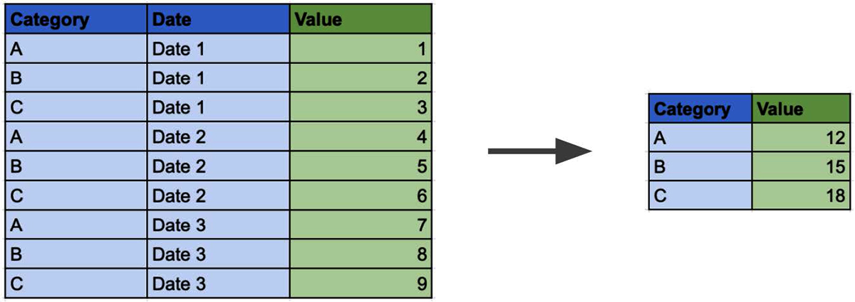
Figure 4-7. An aggregation

Note

Aggregations are covered in detail in Chapter 15.

Join

The Join step (Figure 4-8) adds columns to the original data set from additional data source(s).

Figure 4-8. The Join icon showing an inner join

Depending on the join type and join conditions you set, the resulting data set will differ in terms of the number of data fields, as well as the number of rows if the granularity of the two data sources is different. In Figure 4-9, an inner join joins the rows from two tables based on their common category to form one table.

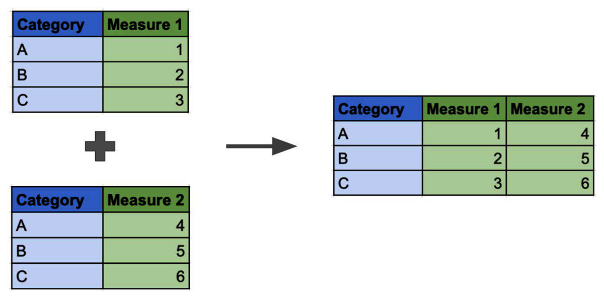
Figure 4-9. An inner join

Note

Joins are covered in more detail in Chapter 16.

Union

The Union step (Figure 4-10) is used to stack data sets on top of each other.

Figure 4-10. The union icon

If the data sets have the same structure with matching data fields, the resulting data set will stay the same width and just include more rows (Figure 4-11).

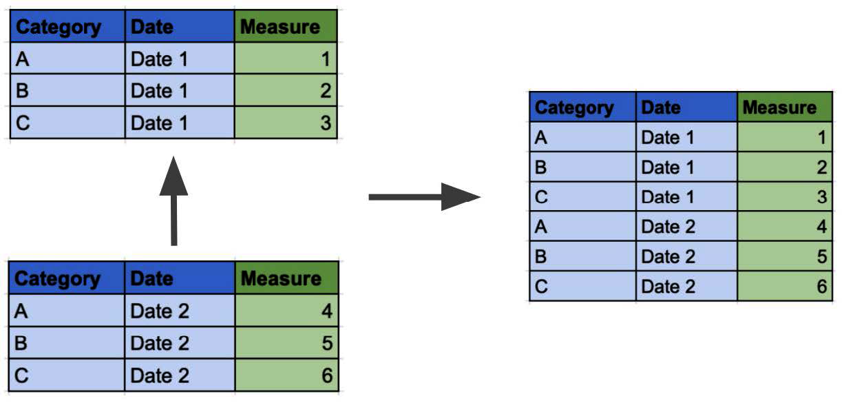
Figure 4-11. Unioning data sets

This step can create a different data structure, as unioning mismatched column headers will create a wider data set. If you don’t merge the mismatched fields, any fields that are not contained in both data sets will have null values.

Note

Unions are covered in more detail in Chapter 17.

Applying Restructuring Techniques to the Ice Cream Example

Let’s apply these data restructuring techniques to the ice cream scents example.

Step 1: Pivot Columns to Rows

Creating a single column to contain dates will allow us to use the data within Desktop more easily, as the date field can be placed on the Columns shelf of Desktop to create an x-axis covering all the dates in the data set. This makes it easy to perform a time-based analysis. This pivot step creates a column labeled Pivot1 Names to hold the former column headers (Figure 4-12). The Pivot1 Names header should be renamed Date for clarity.

Note

Shelves are where you place data in Desktop to analyze it.

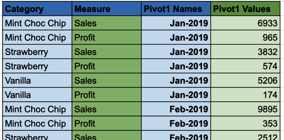
Figure 4-12. The result of the columns-to-rows pivot

Step 2: Pivot Rows to Columns

To create a column for each measure, we need to convert the Measure column values into headers for the new columns containing the relevant sales and profit data (Figure 4-8). The values in these columns will come from the Pivot1 Values column.

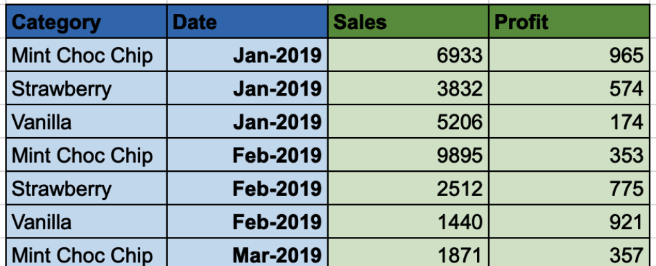
Figure 4-13. The result of the rows-to-columns pivot

Depending on the desired analysis and the tool in which it will be conducted, you might want to aggregate the data at this point up to the category level for each measure. Tableau Desktop can easily aggregate a small data set like this. If no additional data is required from any other tables, no further preparation steps are required for this example.

Summary

As you’ve seen, restructuring data is a key skill to master and practice, as it has made our sample data set much easier to analyze. When manipulating the shape of the data, you must take care to ensure that you haven’t inadvertently duplicated records or changed a measure’s total. Also keep in mind that a longer and thinner data set is not always the intention. A couple of key elements to aim for are:

• A single data field for each dimension, ideally containing a single data type (like a string or date)

• One column per measure

The more closely your data matches this structure, the easier it will be to analyze flexibly, no matter what the subject of the data is. As always, planning your steps before reshaping your data will make the process much easier. As you progress through the following chapters, you will learn more about the importance of reshaping data sets as well as techniques and tactics for doing so that will make your analysis much easier.

¹ This is not the case for Data Interpreter with Excel data sources. The Data Interpreter analyzes the worksheet to return the table(s) of data the sheet contains.

² Prep Builder does not maintain the data source order when loading data. If row order matters, create a row identifier within the data source before loading your data in Prep Builder.