I’m a manager at an engineering company, and I hired an out-of-work political science major to do data entry and other clerical stuff. We don’t pay him a lot, but our deal is that he gets to learn about computers on our dime when he’s doing data entry. There’s only one problem: he types so badly that he makes a ton of mistakes—adding extra numbers, leaving some out, even hitting letters instead of numbers. Isn’t there some way Excel can flag a mistake before he enters the data?
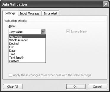
The secret is using data validation. Click a cell (or a group of selected cells), and then turn on the validation feature by selecting Data → Validation and clicking the Settings tab. From the Allow drop-down menu, pick the type of validation criteria you want to use, and then specify its parameters from the drop-down menus that appear below. The type of validation you select in the Allow drop down determines what other options appear below. If you select Whole number, for example, you can specify whether the entered values should be between two other values, not between two other values, or less than or greater than a value. You can hardcode the value by picking “equal to” from the Data drop-down menu and typing the value into the Value field. Figure 1-19shows the types of criteria you can create.
For instance, if he’s supposed to be typing in Zip Codes, and you want to make sure he doesn’t leave out digits or add extra ones, set the Text length validation rule to require a number between 5 and 5. If he’s supposed to enter 94607 and he types 9460 by mistake, he’ll receive an error message reading “The value you entered is not valid.”
If you want to make sure he doesn’t forget to enter data in a critical cell, uncheck the “Ignore blank” box in the Data Validation dialog. That forces him to enter something in the cell. (If you want, you can determine exactly what he needs to enter by selecting the appropriate entry in the Allow drop down.) If the “Ignore blank” box is grayed out, temporarily select anything except “Any value” in the Allow drop down; this makes the “Ignore blank” box accessible. After you uncheck it, you can return to “Any value” if you want, and the “Ignore blank” box, though grayed out, will remain unchecked so that he will have to enter something in the cell.
If you want to keep users from typing data into a cell, you can restrict them to selecting entries from a list. The trick: select List from the Allow drop-down menu. When you do, a field titled Source appears. You can define the list’s values by either selecting a range of cells from the worksheet, or typing values into the Source field, with each one separated by a comma. Entries in the Source field can include spaces, semicolons, and almost any other character. The only character you can’t use is the one that separates entries, i.e., the comma. For example, your list of categories might look like this: Service Plans, Accessories, Sales, On-Site.
I’m a techie in training, but part of the deal I made with my employer is that I must perform a certain amount of data entry drudgery every day before I can learn anything interesting. The problem is that I hate entering data into a worksheet. I make mistakes. I lose my place. Can’t I enter data into something that looks like the paper forms I have stacked right in front of me?
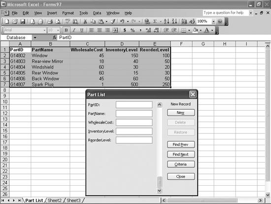
Absolutely! All you need to do is select a data list in your worksheet, and Excel will use it to build a data entry form with an entry field for each item in your list. I guess your next question is probably going to be, “What’s a data list?” I don’t have a definitive answer for Excel 97, 2000, and 2002 (those versions of Excel don’t recognize the concept officially), but I can show you something Excel recognizes as a list, and you can go from there. Figure 1-20 shows you a data list and the resulting data form.
You should note several things about the data in the worksheet:
As you can see in the figure, the headings in the first row of the list (PartID, PartName, and so on) turn into data entry fields.
The columns in the data list either must butt up against the left edge of the worksheet, or there must be a blank column on each side of the data list.
Tip
You can test to see which cells Excel will include in your data list by clicking any cell in what you think is the list and pressing Ctrl-Shift-8. Basically, this tells you which group of cells meets the preceding criteria and which don’t. For you VBA programmers out there, this is the equivalent of calling the ActiveCell.CurrentRegion.Select function when any cell in the list is the active cell.
To create a data entry form, select any cell or group of cells in your heading row and select Data → Form. Excel will create a form like the one in Figure 1-20. Type new data into the form and press Enter or click the New button, and the data is plugged into the worksheet. You can move from field to field in the form by pressing the Tab key, move to the previous field by pressing Shift-Tab, and move through existing data by clicking the Find Prev and Find Next buttons.
Tip
These instructions work if you want to create a data form in Excel 97, 2000, 2002, and 2003. Just remember that in Excel 2003, the term list refers to a data construct that takes advantage of that version’s Extensible Markup Language (XML) capabilities. You’ll learn more about how annoying Excel 2003 (in general) and XML (in particular) can be in Chapter 9.
I use a worksheet to track customer orders, and I’d love to add a validation rule to alert me when customers try to place orders that put them over their credit limit. I know I can create a formula in the cell next to the order total that would do this, but I’d rather use a validation rule so that I’m notified before I finish inputting the order. What’s the secret?
You can use a formula as a validation rule. In this example, we’ll assume the customer’s outstanding balance is in cell C2, the credit limit is in cell C1, and the total price of the new purchase will be entered into cell C3. (You can adjust the formula to work with different layouts.)
Click C3, the cell where the price of the new purchase will be entered.
Select Data → Validation.
Click the Settings tab.
In the Allow drop-down menu, select Custom.
Type =SUM($C$2:$C$3)<=$C$1 into the Formula field, and click OK.
Now if the sum of the new purchase and the outstanding balance exceeds the customer’s credit limit, Excel will display a data validation error message when you try to enter the new purchase.
The dollar signs in front of the column and row references ensure that those cell references won’t change if you copy the formula. If the cell references were written as C2 and so on, the reference would change if you copied the rule to another cell. For more on relative and absolute references, see the annoyance named "Prevent Copied Formulas from Changing Cell References" in Chapter 3.
I have the names of all 50 states in the U.S., plus the District of Columbia, in a list in one worksheet. What’s killing me is that Excel won’t let me use this list as the source for a “Pick from List” validation criterion in a cell on another worksheet! Isn’t there some way to use a set of data from one worksheet as a source of validation criteria in another worksheet?
The trick is to define the list of states as a named range, which you then can refer to in the Data Validation dialog box’s Source field. Here’s how:
Select the cells that contain your valid entries.
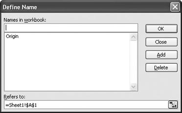
Choose Insert → Name → Define to display the Define Name dialog box (shown in Figure 1-21).
Type a name for the data range in the “Names in workbook” field, click the Add button, and then click OK.
Flip to the other worksheet, select the cells to which you’re adding the validation criteria, and choose Data → Validation.
On the Settings tab, open the Allow drop-down menu and select List.
In the Source field, type an equals sign followed by the name of the named range (e.g., =States)and then click OK. Incidentally, range names are not case-sensitive, so =States and =states are considered the same thing by Excel.
I take inbound calls at a tech-support center, and we track the various callers by recording their phone number in a spreadsheet. The number of different callers is supposedly vital information, and my boss is seriously annoyed if I accidentally enter a caller twice. How can I make sure I avoid duplicate entries in the list?
You can create a data validation criterion that uses a formula to check for previous entries of the same value in the column—but you must prepare the worksheet before you enter any actual data. Here’s how:
In whichever column you want to add the validation criterion (in this example it’s column C) click the second cell (C2 in this case). This example assumes you’re using row 1 for headings; if not, feel free to customize the formula in step 4 to start in a different cell.
Select Data → Validation.
In the Allow drop down, select Custom.
Type =COUNTIF($C$2:$C$65536, C2)=1 in the Formula field, and click OK.
Grab the fill handle, and drag from cell C2 down as far as you want your no-duplicates validation rule to apply.
This formula starts by noting the value in cell C2 and counts the number of times the value occurs in the range $C$2:$C$65536. Because the formula checks the value in the active cell, there will always be at least one occurrence. However, if Excel finds two occurrences the program recognizes the value is a duplicate and rejects it.
Because of the way the cell designations are written, as you drag the formula down from cell C2, the range $C$2:$C$65536 remains constant from cell to cell because of the dollar signs in front of the column and row references. (For more information on relative and absolute references, see the annoyance named "Prevent Copied Formulas from Changing Cell References" in Chapter 3.) But C2 changes to C3 in cell C3, to C4 in cell C4, and so on. I chose the range $C$2:$C$65536 because an Excel worksheet can have up to 65,536 rows, so that range covers ‘em all.
I give each of my data entry staffers a printout listing the validation criteria for each cell in my workbook. But I’m still getting complaints because after a week or two they misplace the printout, and then when they enter the wrong data all the Excel error message says is: “The value you entered is not valid. A user has restricted values that can be entered into this cell.” This is stupid! Isn’t there some way I can get Excel to provide more specific error messages?
Sure thing. You can create custom messages when you create your validation rules. The Data Validation dialog box has three tabs: Settings (which you use to create the validation rule), Input Message (which lets you display a dialog box when a user clicks a cell with the validation rule), and Error Alert (which displays various different alert boxes when the user attempts to enter an invalid value into the cell). So, there are actually two ways to skin your cat: using an input message or using an error alert.
You can use an input message to remind your data entry people what’s supposed to go in a given cell. Here’s how:
Click the cell you want to modify.
Choose Data → Validation, and click the Input Message tab.
Check the “Show input message when cell is selected” box.
Type a title and an input message in the fields provided. For instance, your message could say “Zip Codes only.”
The only trouble with input messages is that they pop up every time a user enters a cell, even if they already remember what kind of data goes there. This can be, um, annoying.
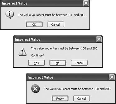
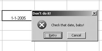
If you prefer to correct users after they actually make a mistake, use the error alert box. There are three types of error alert boxes: Information, Warning, and Stop. (Figure 1-22 shows the three different styles of error alert boxes.) Here’s how each one operates:
Figure 1-22. The type of error alert box you create determines whether a user can ignore your criteria.
-
Information This box offers the user two choices: OK, which closes the dialog box, enters the invalid data, and moves the cell pointer to the next cell; and Cancel, which deletes the entry and keeps the pointer in the same cell. Unless you make the Title and Error Message text very specific, an information box can simply confuse the user more. For instance, it will help if the title reads something like “You were supposed to enter five numbers!” and the error message reads along the lines of “Clicking OK will enter the invalid data. Clicking Cancel will delete the entry and let you try again.”
-
Warning This error alert box, by contrast, indicates that the user has entered invalid data and asks if he wants to continue. The box has three buttons: Yes, which closes the dialog box, enters the invalid data, and moves the cell pointer to the next cell; No, which returns the user to the cell with the cell’s contents highlighted; and Cancel, which deletes the entry and keeps the pointer on the same cell. As with the Information box, providing a helpful text message is a must.
-
Stop This type of error alert box makes it impossible for the user to leave the cell while it contains invalid data (see Figure 1-23). The Stop box has two buttons: Retry, which returns the user to the cell with the cell’s contents highlighted; and Cancel, which deletes the entry and keeps the pointer on the same cell. As in the two preceding examples, providing a helpful text message is a must.
To create an error alert box, follow these steps:
Click the cell you want to modify.
Choose Data → Validation, and click the Error Alert tab.
Make sure the “Show error alert after invalid data is entered” box is checked.
From the Style drop down, select the type of alert you want to create, enter text for the title and error message in the fields provided, and click OK.
I provide IT support for a building supply company, and one of my prime responsibilities is maintaining a spreadsheet with lots of customer information, including credit limits. Over the last six months I’ve entered several hundred records, but I just found out the minimum credit limit is supposed to be $1,000—and I know some of the customer records I entered listed credit limits lower than that. I added a validation rule to every cell in the column, requiring a number 1,000 or higher, hoping Excel would display all the cells with invalid data, but nothing happened. Do I have to go through the worksheet row by row to find values lower than $1,000? There’s gotta be a faster way to find invalid data!
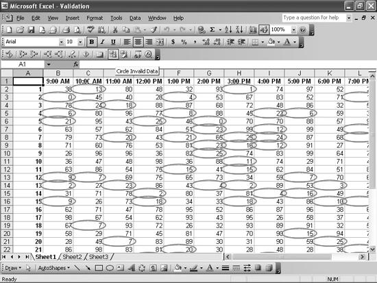
In Excel 97 and 2000, you can tell Excel to circle any cells with invalid data by choosing Tools → Auditing → Show Auditing Toolbar. On the Auditing toolbar, click the Circle Invalid Data button to draw a red circle around any cell that contains invalid data (as shown in Figure 1-24).
In Excel 2002 and 2003 the menu items have changed a bit, but the process is basically the same: choose Tools → Formula Auditing → Show Formula Auditing Toolbar. On the Formula Auditing toolbar, click the Circle Invalid Data button to draw a red circle around any cells that contain invalid data.
To remove the circles, click the Clear Validation Circles button on the Formula Auditing toolbar.
I use Excel to track the hours volunteers work at a hospital. I created a named range that contains all their names, and I use that range as the source for my List validation rule. The problem is that I want to copy the validation rule, and just the validation rule, to another cell in my worksheet instead of having to re-create it. Please tell me there’s a way to do that!
To copy the validation rule from one cell to another, follow these steps:
Select the cell containing the validation rule, and choose Edit → Copy.
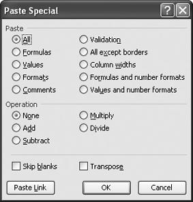
Select the target cells and choose Edit → Paste Special to display the Paste Special dialog box (shown in Figure 1-25).
Select Validation and click OK.
In every Windows version of Excel I’ve ever used, when I’m scrolling down through a workbook the scroll starts nice and slow for a second or two...before kicking into warp speed and leaving me thousands of rows further down than I wanted to be. How do I keep Excel from going turbo?
This is a known bug in Excel 2002 and earlier versions. Microsoft finally fixed it in Excel 2003, but that doesn’t help anyone with an earlier edition. If you have a wheel mouse, no problem: just use the wheel to scroll down at a perfectly controllable speed. If you don’t have a wheel mouse, this is a perfect excuse to buy one! Come on, they’re cheap!
If you insist on working with an older mouse, and still want to limit Excel’s scrolling speed, I recommend clicking the scrollbar just above or below the slider to move up or down one screen at a time (the equivalent keyboard commands are Page Up and Page Down). Pressing Alt-Page Up moves you one screen to the left, while pressing Alt-Page Down moves you one screen to the right.
Get Excel Annoyances now with the O’Reilly learning platform.
O’Reilly members experience books, live events, courses curated by job role, and more from O’Reilly and nearly 200 top publishers.
