book

Microscope Image Processing

Name: Microscope Image Processing
ISBN: 9780080558547

by Qiang Wu, Fatima Merchant, Kenneth Castleman

July 2010

Intermediate to advanced

576 pages

17h 29m

English

Academic Press

Read now

Unlock full access

Front Cover
Microscope Image Processing
Copyright Page
Contents (1/4)
Contents (2/4)
Contents (3/4)
Contents (4/4)
Foreword
Reference
Preface

Acknowledgments
Chapter 1: Introduction
1.1 The Microscope and Image Processing1.2 Scope of This Book
1.3 Our Approach
1.3.1 The Four Types of Images1.3.1.1 Optical Image1.3.1.2 Continuous Image1.3.1.3 Digital Image
1.3.1.4 Displayed Image
1.3.2 The Result1.3.2.1 Analytic Functions
1.3.3 The Sampling Theorem
1.4 The Challenge
1.5 Nomenclature1.6 Summary of Important Points
References
Chapter 2: Fundamentals of Microscopy
2.1 Origins of the Microscope
2.2 Optical Imaging
2.2.1 Image Formation by a Lens2.2.1.1 Imaging a Point Source2.2.1.2 Focal Length2.2.1.3 Numerical Aperture
2.2.1.4 Lens Shape
2.3 Diffraction-Limited Optical Systems
2.3.1 Linear System Analysis
2.4 Incoherent Illumination2.4.1 The Point Spread Function
2.4.2 The Optical Transfer Function
2.5 Coherent Illumination
2.5.1 The Coherent Point Spread Function
2.5.2 The Coherent Optical Transfer Function
2.6 Resolution
2.6.1 Abbe Distance
2.6.2 Rayleigh Distance2.6.3 Size Calculations
2.7 Aberration
2.8 Calibration
2.8.1 Spatial Calibration
2.8.2 Photometric Calibration
2.9 Summary of Important Points
References
Chapter 3: Image Digitization
3.1 Introduction
3.2 Resolution
3.3 Sampling
3.3.1 Interpolation
3.3.2 Aliasing
3.4 Noise
3.5 Shading
3.6 Photometry
3.7 Geometric Distortion
3.8 Complete System Design3.8.1 Cumulative Resolution
3.8.2 Design Rules of Thumb
3.8.2.1 Pixel Spacing3.8.2.2 Resolution3.8.2.3 Noise3.8.2.4 Photometry
3.8.2.5 Distortion
3.9 Summary of Important PointsReferences
Chapter 4: Image Display
4.1 Introduction
4.2 Display Characteristics
4.2.1 Displayed Image Size4.2.2 Aspect Ratio
4.2.3 Photometric Resolution
4.2.4 Grayscale Linearity
4.2.5 Low-Frequency Response4.2.5.1 Pixel Polarity
4.2.5.2 Pixel Interaction
4.2.6 High-Frequency Response4.2.7 The Spot-Spacing Compromise4.2.8 Noise Considerations
4.3 Volatile Displays
4.4 Sampling for Display Purposes
4.4.1 Oversampling
4.4.2 Resampling
4.5 Display Calibration
4.6 Summary of Important Points
References
Chapter 5: Geometric Transformations
5.1 Introduction
5.2 Implementation
5.3 Gray-Level Interpolation
5.3.1 Nearest-Neighbor Interpolation
5.3.2 Bilinear Interpolation
5.3.3 Bicubic Interpolation
5.3.4 Higher-Order Interpolation
5.4 Spatial Transformation
5.4.1 Control-Grid Mapping
5.5 Applications
5.5.1 Distortion Removal5.5.2 Image Registration5.5.3 Stitching
5.6 Summary of Important Points
References
Chapter 6: Image Enhancement
6.1 Introduction
6.2 Spatial Domain Methods
6.2.1 Contrast Stretching
6.2.2 Clipping and Thresholding
6.2.3 Image Subtraction and Averaging
6.2.4 Histogram Equalization
6.2.5 Histogram Specification
6.2.6 Spatial Filtering
6.2.7 Directional and Steerable Filtering
6.2.8 Median Filtering
6.3 Fourier Transform Methods
6.3.1 Wiener Filtering and Wiener Deconvolution
6.3.2 Deconvolution Using a Least-Squares Approach
6.3.3 Low-Pass Filtering in the Fourier Domain
6.3.4 High-Pass Filtering in the Fourier Domain
6.4 Wavelet Transform Methods
6.4.1 Wavelet Thresholding
6.4.2 Differential Wavelet Transform and Multiscale Pointwise Product
6.5 Color Image Enhancement
6.5.1 Pseudo-Color Transformations
6.5.2 Color Image Smoothing6.5.3 Color Image Sharpening
6.6 Summary of Important Points
References
Chapter 7: Wavelet Image Processing
7.1 Introduction
7.1.1 Linear Transformations
7.1.2 Short-Time Fourier Transform and Wavelet Transform
7.2 Wavelet Transforms
7.2.1 Continuous Wavelet Transform
7.2.2 Wavelet Series Expansion
7.2.3 Haar Wavelet Functions
7.3 Multiresolution Analysis
7.3.1 Multiresolution and Scaling Function
7.3.2 Scaling Functions and Wavelets
7.4 Discrete Wavelet Transform
7.4.1 Decomposition
7.4.2 Reconstruction
7.4.3 Filter Banks
7.4.3.1 Two-Channel Subband Coding7.4.3.2 Orthogonal Filter Design
7.4.4 Compact Support
7.4.5 Biorthogonal Wavelet Transforms
7.4.5.1 Biorthogonal Filter Banks7.4.5.2 Examples of Biorthogonal Wavelets
7.4.6 Lifting Schemes
7.4.6.1 Biorthogonal Wavelet Design7.4.6.2 Wavelet Transform Using Lifting
7.5 Two-Dimensional Discrete Wavelet Transform
7.5.1 Two-Dimensional Wavelet Bases
7.5.2 Forward Transform
7.5.3 Inverse Transform
7.5.4 Two-Dimensional Biorthogonal Wavelets
7.5.5 Overcomplete Transforms
7.6 Examples
7.6.1 Image Compression7.6.2 Image Enhancement
7.6.3 Extended Depth-of-Field by Wavelet Image Fusion
7.7 Summary of Important Points
References
Chapter 8: Morphological Image Processing
8.1 Introduction
8.2 Binary Morphology
8.2.1 Binary Erosion and Dilation
8.2.2 Binary Opening and Closing
8.2.3 Binary Morphological Reconstruction from Markers
8.2.3.1 Connectivity8.2.3.2 Markers
8.2.3.3 The Edge-Off Operation
8.2.4 Reconstruction from Opening
8.2.5 Area Opening and Closing
8.2.6 Skeletonization
8.3 Grayscale Operations
8.3.1 Threshold Decomposition
8.3.2 Erosion and Dilation
8.3.2.1 Gradient
8.3.3 Opening and Closing8.3.3.1 Top-Hat Filtering8.3.3.2 Alternating Sequential Filters
8.3.4 Component Filters and Grayscale Morphological Reconstruction
8.3.4.1 Morphological Reconstruction8.3.4.2 Alternating Sequential Component Filters8.3.4.3 Grayscale Area Opening and Closing8.3.4.4 Edge-Off Operator8.3.4.5 h-Maxima and h-Minima Operations8.3.4.6 Regional Maxima and Minima
8.3.4.7 Regional Extrema as Markers
8.4 Watershed Segmentation
8.4.1 Classical Watershed Transform
8.4.2 Filtering the Minima
8.4.3 Texture Detection
8.4.4 Watershed from Markers
8.4.5 Segmentation of Overlapped Convex Cells
8.4.6 Inner and Outer Markers
8.4.7 Hierarchical Watershed
8.4.8 Watershed Transform Algorithms
8.5 Summary of Important Points
References
Chapter 9: Image Segmentation
9.1 Introduction
9.1.1 Pixel Connectivity
9.2 Region-Based Segmentation9.2.1 Thresholding9.2.1.1 Global Thresholding9.2.1.2 Adaptive Thresholding9.2.1.3 Threshold Selection
9.2.1.4 Thresholding Circular Spots
9.2.1.5 Thresholding Noncircular and Noisy Spots
9.2.2 Morphological Processing
9.2.2.1 Hole Filling9.2.2.2 Border-Object Removal9.2.2.3 Separation of Touching Objects9.2.2.4 The Watershed Algorithm
9.2.3 Region Growing
9.2.4 Region Splitting
9.3 Boundary-Based Segmentation
9.3.1 Boundaries and Edges
9.3.2 Boundary Tracking Based on Maximum Gradient Magnitude
9.3.3 Boundary Finding Based on Gradient Image Thresholding
9.3.4 Boundary Finding Based on Laplacian Image Thresholding
9.3.5 Boundary Finding Based on Edge Detection and Linking (1/2)
9.3.5.1 Edge Detection9.3.5.2 Edge Linking and Boundary Refinement
9.3.5 Boundary Finding Based on Edge Detection and Linking (2/2)
9.3.6 Encoding Segmented Images
9.3.6.1 Object Label Map9.3.6.2 Boundary Chain Code
9.4 Summary of Important Points
References
Chapter 10: Object Measurement
10.1 Introduction
10.2 Measures for Binary Objects
10.2.1 Size Measures10.2.1.1 Area10.2.1.2 Perimeter10.2.1.3 Area and Perimeter of a Polygon
10.2.2 Pose Measures
10.2.2.1 Centroid
10.2.2.2 Orientation
10.2.3 Shape Measures (1/2)10.2.3.1 Thinness Ratio10.2.3.2 Rectangularity10.2.3.3 Circularity10.2.3.4 Euler Number10.2.3.5 Moments
10.2.3 Shape Measures (2/2)
10.2.3.6 Elongation
10.2.4 Shape Descriptors
10.2.4.1 Differential Chain Code10.2.4.2 Fourier Descriptors10.2.4.3 Medial Axis Transform10.2.4.4 Graph Representations
10.3 Distance Measures
10.3.1 Euclidean Distance10.3.2 City-Block Distance
10.3.3 Chessboard Distance
10.4 Gray-Level Object Measures10.4.1 Intensity Measures10.4.1.1 Integrated Optical Intensity10.4.1.2 Average Optical Intensity
10.4.1.3 Contrast
10.4.2 Histogram Measures10.4.2.1 Mean Gray Level10.4.2.2 Standard Deviation of Gray Levels
10.4.2.3 Skew
10.4.2.4 Entropy10.4.2.5 Energy10.4.3 Texture Measures10.4.3.1 Statistical Texture Measures10.4.3.2 Power Spectrum Features
10.5 Object Measurement Considerations
10.6 Summary of Important Points
References
Chapter 11: Object Classification
11.1 Introduction11.2 The Classification Process
11.2.1 Bayes’ Rule
11.3 The Single-Feature, Two-Class Case
11.3.1 A Priori Probabilities
11.3.2 Conditional Probabilities
11.3.3 Bayes’ Theorem
11.4 The Three-Feature, Three-Class Case
11.4.1 Bayes Classifier
11.4.1.1 Prior Probabilities11.4.1.2 Classifier Training11.4.1.3 The Mean Vector11.4.1.4 Covariance11.4.1.5 Variance and Standard Deviation11.4.1.6 Correlation11.4.1.7 The Probability Density Function11.4.1.8 Classification11.4.1.9 Log Likelihoods11.4.1.10 Mahalanobis Distance Classifier11.4.1.11 Uncorrelated Features
11.4.2 A Numerical Example
11.5 Classifier Performance
11.5.1 The Confusion Matrix
11.6 Bayes Risk
11.6.1 Minimum-Risk Classifier
11.7 Relationships Among Bayes Classifiers
11.8 The Choice of a Classifier
11.8.1 Subclassing
11.8.2 Feature Normalization
11.9 Nonparametric Classifiers
11.9.1 Nearest-Neighbor Classifiers
11.10 Feature Selection
11.10.1 Feature Reduction11.10.1.1 Principal Component Analysis11.10.1.2 Linear Discriminant Analysis
11.11 Neural Networks
11.12 Summary of Important Points
References
Chapter 12: Fluorescence Imaging
12.1 Introduction
12.2 Basics of Fluorescence Imaging
12.2.1 Image Formation in Fluorescence Imaging
12.3 Optics in Fluorescence Imaging
12.4 Limitations in Fluorescence Imaging
12.4.1 Instrumentation-Based Aberrations12.4.1.1 Photon Shot Noise12.4.1.2 Dark Current12.4.1.3 Auxiliary Noise Sources
12.4.1.4 Quantization Noise
12.4.1.5 Other Noise Sources12.4.2 Sample-Based Aberrations12.4.2.1 Photobleaching12.4.2.2 Autofluorescence
12.4.2.3 Absorption and Scattering
12.4.3 Sample and Instrumentation Handling–Based Aberrations
12.5 Image Corrections in Fluorescence Microscopy
12.5.1 Background Shading Correction
12.5.2 Correction Using the Recorded Image
12.5.3 Correction Using Calibration Images
12.5.3.1 Two-Image Calibration12.5.3.2 Background Subtraction
12.5.4 Correction Using Surface Fitting
12.5.5 Histogram-Based Background Correction
12.5.6 Other Approaches for Background Correction12.5.7 Autofluorescence Correction
12.5.8 Spectral Overlap Correction
12.5.9 Photobleaching Correction
12.5.10 Correction of Fluorescence Attenuation in Depth
12.6 Quantifying Fluorescence
12.6.1 Fluorescence Intensity Versus Fluorophore Concentration
12.7 Fluorescence Imaging Techniques
12.7.1 Immunofluorescence
12.7.2 Fluorescence in situ Hybridization (FISH)
12.7.3 Quantitative Colocalization Analysis
12.7.4 Fluorescence Ratio Imaging (RI)
12.7.5 Fluorescence Resonance Energy Transfer (FRET) (1/2)
12.7.5 Fluorescence Resonance Energy Transfer (FRET) (2/2)
12.7.6 Fluorescence Lifetime Imaging (FLIM)
12.7.7 Fluorescence Recovery After Photobleaching (FRAP)
12.7.8 Total Internal Reflectance Fluorescence Microscopy (TIRFM)
12.7.9 Fluorescence Correlation Spectroscopy (FCS)
12.8 Summary of Important Points
References (1/2)
References (2/2)
Chapter 13: Multispectral Imaging
13.1 Introduction
13.2 Principles of Multispectral Imaging
13.2.1 Spectroscopy
13.2.2 Imaging
13.2.3 Multispectral Microscopy
13.2.4 Spectral Image Acquisition Methods13.2.4.1 Wavelength-Scan Methods13.2.4.2 Spatial-Scan Methods
13.2.4.3 Time-Scan Methods
13.3 Multispectral Image Processing
13.3.1 Calibration for Multispectral Image Acquisition
13.3.2 Spectral Unmixing (1/2)
13.3.2.1 Fluorescence Unmixing
13.3.2 Spectral Unmixing (2/2)
13.3.2.2 Brightfield Unmixing13.3.2.3 Unsupervised Unmixing
13.3.3 Spectral Image Segmentation
13.3.3.1 Combining Segmentation with Classification13.3.3.2 M-FISH Pixel Classification
13.4 Summary of Important Points
References
Chapter 14: Three-Dimensional Imaging
14.1 Introduction14.2 Image Acquisition
14.2.1 Wide-Field Three-Dimensional Microscopy
14.2.2 Confocal Microscopy
14.2.3 Multiphoton Microscopy
14.2.4 Other Three-Dimensional Microscopy Techniques
14.3 Three-Dimensional Image Data
14.3.1 Three-Dimensional Image Representation14.3.1.1 Three-Dimensional Image Notation
14.4 Image Restoration and Deblurring
14.4.1 The Point Spread Function14.4.1.1 Theoretical Model of the Point Spread Function
14.4.2 Models for Microscope Image Formation
14.4.2.1 Poisson Noise14.4.2.2 Gaussian Noise
14.4.3 Algorithms for Deblurring and Restoration (1/4)
14.4.3.1 No-Neighbor Methods14.4.3.2 Nearest-Neighbor Method14.4.3.3 Linear Methods
14.4.3 Algorithms for Deblurring and Restoration (2/4)
14.4.3.4 Nonlinear Methods
14.4.3 Algorithms for Deblurring and Restoration (3/4)
14.4.3.5 Maximum-Likelihood Restoration14.4.3.6 Blind Deconvolution
14.4.3 Algorithms for Deblurring and Restoration (4/4)
14.4.3.7 Interpretation of Deconvolved Images14.4.3.8 Commercial Deconvolution Packages
14.5 Image Fusion
14.6 Three-Dimensional Image Processing
14.7 Geometric Transformations
14.8 Pointwise Operations
14.9 Histogram Operations
14.10 Filtering
14.10.1 Linear Filters14.10.1.1 Finite Impulse Response (FIR) Filter
14.10.2 Nonlinear Filters
14.10.2.1 Median Filter14.10.2.2 Weighted Median Filter
14.10.2.3 Minimum and Maximum Filters
14.10.2.4 alpha-Trimmed Mean Filters14.10.3 Edge-Detection Filters
14.11 Morphological Operators
14.11.1 Binary Morphology
14.11.2 Grayscale Morphology
14.12 Segmentation
14.12.1 Point-Based Segmentation
14.12.2 Edge-Based Segmentation
14.12.3 Region-Based Segmentation
14.12.3.1 Connectivity14.12.3.2 Region Growing14.12.3.3 Region Splitting and Region Merging
14.12.4 Deformable Models
14.12.5 Three-Dimensional Segmentation Methods in the Literature
14.13 Comparing Three-Dimensional Images
14.14 Registration
14.15 Object Measurements in Three Dimensions
14.15.1 Euler Number
14.15.2 Bounding Box
14.15.3 Center of Mass
14.15.4 Surface Area Estimation
14.15.5 Length Estimation
14.15.6 Curvature Estimation
14.15.6.1 Surface Triangulation Method
14.15.6.2 Cross-Patch Method14.15.7 Volume Estimation
14.15.8 Texture
14.16 Three-Dimensional Image Display14.16.1 Montage
14.16.2 Projected Images
14.16.2.1 Voxel Projection14.16.2.2 Ray Casting
14.16.3 Surface and Volume Rendering
14.16.3.1 Surface Rendering14.16.3.2 Volume Rendering
14.16.4 Stereo Pairs
14.16.5 Color Anaglyphs
14.16.6 Animations
14.17 Summary of Important Points
References (1/2)
References (2/2)
Chapter 15: Time-Lapse Imaging
15.1 Introduction
15.2 Image Acquisition
15.2.1 Microscope Setup
15.2.2 Spatial Dimensionality
15.2.3 Temporal Resolution
15.3 Image Preprocessing
15.3.1 Image Denoising
15.3.2 Image Deconvolution
15.3.3 Image Registration
15.4 Image Analysis
15.4.1 Cell Tracking
15.4.1.1 Cell Segmentation
15.4.1.2 Cell Association
15.4.2 Particle Tracking15.4.2.1 Particle Detection15.4.2.2 Particle Association
15.5 Trajectory Analysis
15.5.1 Geometry Measurements
15.5.2 Diffusivity Measurements
15.5.3 Velocity Measurements
15.6 Sample Algorithms
15.6.1 Cell Tracking
15.6.2 Particle Tracking
15.7 Summary of Important Points
References (1/2)
References (2/2)
Chapter 16: Autofocusing
16.1 Introduction16.1.1 Autofocus Methods
16.1.2 Passive Autofocusing
16.2 Principles of Microscope Autofocusing
16.2.1 Fluorescence and Brightfield Autofocusing
16.2.2 Autofocus Functions
16.2.3 Autofocus Function Sampling and Approximation
16.2.3.1 Gaussian Fitting16.2.3.2 Parabola Fitting
16.2.4 Finding the In-Focus Imaging Position
16.3 Multiresolution Autofocusing
16.3.1 Multiresolution Image Representations
16.3.2 Wavelet-Based Multiresolution Autofocus Functions
16.3.3 Multiresolution Search for In-Focus Position
16.4 Autofocusing for Scanning Microscopy
16.5 Extended Depth-of-Field Microscope Imaging
16.5.1 Digital Image Fusion
16.5.2 Pixel-Based Image Fusion
16.5.3 Neighborhood-Based Image Fusion
16.5.4 Multiresolution Image Fusion
16.5.5 Noise and Artifact Control in Image Fusion
16.5.5.1 Multiscale Pointwise Product16.5.5.2 Consistency Checking
16.5.5.3 Reassignment
16.6 Examples16.7 Summary of Important Points
References
Chapter 17: Structured Illumination Imaging
17.1 Introduction17.1.1 Conventional Light Microscope
17.1.2 Sectioning the Specimen
17.1.3 Structured Illumination
17.2 Linear SIM Instrumentation
17.2.1 Spatial Light Modulator
17.3 The Process of Structured Illumination Imaging
17.3.1 Extended-Depth-of-Field Image
17.3.2 SIM for Optical Sectioning
17.3.3 Sectioning Strength
17.4 Limitations of Optical Sectioning with SIM
17.4.1 Artifact Reduction via Image Processing (1/2)
17.4.1.1 Intensity Normalization17.4.1.2 Grid Position Error17.4.1.3 Statistical Waveform Compensation
17.4.1 Artifact Reduction via Image Processing (2/2)
17.4.1.4 Parameter Optimization
17.5 Color Structured Illumination
17.5.1 Processing Technique
17.5.2 Chromatic Aberration
17.5.3 SIM Example
17.6 Lateral Superresolution
17.6.1 Bypassing the Optical Transfer Function
17.6.2 Mathematical Foundation
17.6.2.1 Shifting Frequency Space17.6.2.2 Extracting the Enhanced Image
17.6.3 Lateral Resolution Enhancement Simulation
17.7 Summary of Important Points
References
Chapter 18: Image Data and Workflow Management
18.1 Introduction
18.1.1 Open Microscopy Environment
18.1.2 Image Management in Other Fields18.1.3 Requirements for Microscopy Image Management Systems
18.2 Architecture of Microscopy Image/Data/Workflow Systems
18.2.1 Client–Server Architecture
18.2.2 Image and Data Servers
18.2.3 Users, Ownership, Permissions
18.3 Microscopy Image Management
18.3.1 XYZCT Five-Dimensional Imaging Model18.3.2 Image Viewers
18.3.3 Image Hierarchies
18.3.3.1 Predefined Containers18.3.3.2 User-Defined Containers
18.3.4 Browsing and Search
18.3.5 Microscopy Image File Formats and OME-XML
18.3.5.1 OME-XML Image Acquisition Ontology
18.4 Data Management
18.4.1 Biomedical Ontologies
18.4.2 Building Ontologies with OME SemanticTypes
18.4.3 Data Management Software with Plug-in Ontologies
18.4.4 Storing Data with Ontological Structure
18.4.4.1 Image Acquisition Meta-Data18.4.4.2 Mass Annotations18.4.4.3 Spreadsheet Annotations
18.5 Workflow Management
18.5.1 Data Provenance18.5.1.1 OME AnalysisModules18.5.1.2 Editing and Deleting Data
18.5.2 Modeling Quantitative Image Analysis (1/2)
18.5.2.1 Coupling Algorithms to Informatics Platforms18.5.2.2 Composing Workflows18.5.2.3 Enacting Workflows
18.5.2 Modeling Quantitative Image Analysis (2/2)
18.6 Summary of Important Points
References
Glossary of Microscope Image Processing Terms (1/2)
Glossary of Microscope Image Processing Terms (2/2)
References
Index (1/2)
Index (2/2)
Color Plate Section (1/2)
Color Plate Section (2/2)

Content preview from Microscope Image Processing

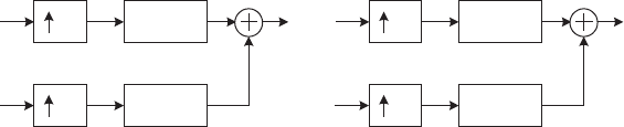
the results are then added to reconstruct c

jþ1

. Figure 7.6 illustrates this recon-

struction (synthesis) procedure, or the inverse DWT.

As is seen from Eq. 7.43, the same digital ﬁlters used in the analysis are used

for the synthesis, since we have deﬁned orthonormal scaling and wavelet func-

tions. This type of transformation is known as an orthogonal (or, more specif-

ically, orthonormal ) discrete wavelet transform. If the analysis and synthesis

ﬁlters are different but the transform is invertible, then the transform is known

as a biorthogonal wavelet transform, as explained later in this chapter. Due

to this orthonormality, g

(n) ¼ h

(n) and

Become an O’Reilly member and get unlimited access to this title plus top books and audiobooks from O’Reilly and nearly 200 top publishers, thousands of courses curated by job role, 150+ live events each month,
and much more.

Read now

Unlock full access

More than 5,000 organizations count on O’Reilly

O’Reilly covers everything we've got, with content to help us build a world-class technology community, upgrade the capabilities and competencies of our teams, and improve overall team performance as well as their engagement.

Julian F.

Head of Cybersecurity

I wanted to learn C and C++, but it didn't click for me until I picked up an O'Reilly book. When I went on the O’Reilly platform, I was astonished to find all the books there, plus live events and sandboxes so you could play around with the technology.

Addison B.

Field Engineer

I’ve been on the O’Reilly platform for more than eight years. I use a couple of learning platforms, but I'm on O'Reilly more than anybody else. When you're there, you start learning. I'm never disappointed.

Amir M.

Data Platform Tech Lead

I'm always learning. So when I got on to O'Reilly, I was like a kid in a candy store. There are playlists. There are answers. There's on-demand training. It's worth its weight in gold, in terms of what it allows me to do.

Mark W.

Embedded Software Engineer

Computational Vision and Medical Image Processing IV

Publisher Resources

ISBN: 9780080558547

Cloud Computing

Data Engineering

Data Science

AI & ML

Programming Languages

Software Architecture

IT/Ops

Security

Design

Business

Soft Skills

Microscope Image Processing

by Qiang Wu, Fatima Merchant, Kenneth Castleman

Become an O’Reilly member and get unlimited access to this title plus top books and audiobooks from O’Reilly and nearly 200 top publishers, thousands of courses curated by job role, 150+ live events each month,
and much more.

More than 5,000 organizations count on O’Reilly

Julian F.

Addison B.

Amir M.

Mark W.

You might also like

Computational Vision and Medical Image Processing IV

Feature Extraction and Image Processing

Machine Vision Inspection Systems, Image Processing, Concepts, Methodologies, and Applications

Handbook of Optical Metrology, 2nd Edition

Publisher Resources