The R Book

Comparing Michaelis–Menten and Asymptotic Exponential

Model choice is always an important issue in curve fitting. We shall compare the fit of the asymptotic exponential (above) with a Michaelis–Menten with parameter values estimated from the same deer jaws data. As to starting values for the parameters, it is clear that a reasonable estimate for the asymptote would be 100 (this is a/b; see p. 202). The curve passes close to the point (5, 40) so we can guess a value of a of 40/5 = 8 and hence b = 8/100 = 0.08. Now use nls to estimate the parameters:

(model3<-nls(bone~a*age/(1+b*age),start=list(a=8,b=0.08)))

Nonlinear regression model
  model: bone~a * age/(1 + b * age)

data: parent.frame()
         a          b
18.7253859  0.1359640
residual sum-of-squares: 9854.409

Finally, we can add the line for Michaelis–Menten to the original plot. You could draw the best-fit line by transcribing the parameter values

ymm<-18.725*av/(1+0.13596*av)
lines(av,ymm,lty=2)

Alternatively, you could use predict with the model name, using list to allocate x values to age:

ymm<-predict(model3, list(age=av))
lines(av,ymm,lty=2)

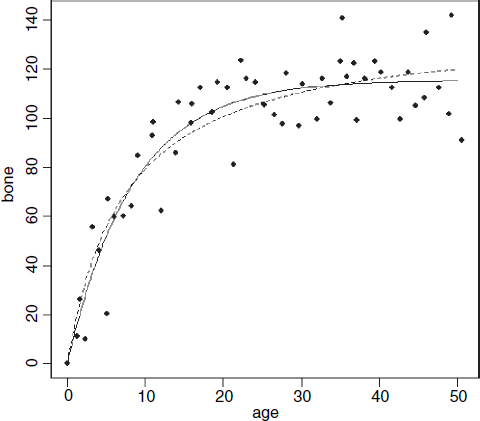
You can see that the asymptotic exponential (solid line) tends to get to its asymptote first, and that the Michaelis–Menten (dotted line) continues to increase. Model choice, therefore would be enormously important if you intended to use the model for prediction to ages much greater than 50 months. ...