The R Book

Generalized Additive Models

Sometimes we can see that the relationship between yand x is non-linear but we don't have any theory or any mechanistic model to suggest a particular functional form (mathematical equation) to describe the relationship. In such circumstances, generalized additive models GAMs are particularly useful because they fit non-parametric smoothers to the data without requiring us to specify any particular mathematical model to describe the non-linearity (background and more examples are given in Chapter 18).

humped<-read.table("c:\\temp\\hump.txt",header=T)
attach(humped)
names(humped)

[1] "y" "x"

plot(x,y,pch=16)
library(mgcv)

The model is specified very simply by showing which explanatory variables (in this case just x) are to be fitted as smoothed functions using the notation y~s(x):

model<-gam(y~s(x))

Now we can use predict in the normal way to fit the curve estimated by gam:

xv<-seq(0.5,1.3,0.01)
yv<-predict(model,list(x=xv))
lines(xv,yv)

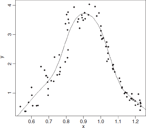
summary(model)

Family: gaussian
Link function: identity

Formula:
y ~ s(x)

Parametric coefficients:
            Estimate  Std. Error  t value  Pr(>|t|)
(Intercept)  1.95737     0.03446     56.8    <2e-16    ***

Approximate significance of smooth terms:
        edf  Est.rank      F   p-value
s(x)  7.452         9  110.0    <2e-16    ***

R-sq.(adj) = 0.919  Deviance explained = 92.6%
GCV score = 0.1156  Scale est. = 0.1045  n = 88

Fitting the curve uses up 7.452 degrees of freedom ...