Pythonデータサイエンスハンドブック ―Jupyter、NumPy、pandas、Matplotlib、scikit-learnを使ったデータ分析、機械学習

4.7

 ヒストグラム、ビニング、密度

249

plt.hist

の

docstring

には、その他のカスタマイズオプションが数多く解説されています。異

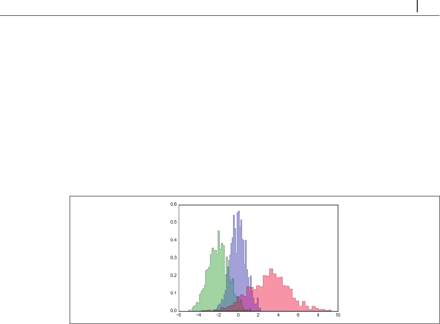
なる分布のヒストグラムを比較する際には、

histtype='stepfilled'

オプションを使い、透過度

alpha

を設定すると見やすいグラフになります（図 4-37）。

In[4]: x1 = np.random.normal(0, 0.8, 1000)

x2 = np.random.normal(-2, 1, 1000)

x3 = np.random.normal(3, 2, 1000)

kwargs = dict(histtype='stepfilled', alpha=0.3, normed=True, bins=40)

plt.hist(x1, **kwargs)

plt.hist(x2,

**kwargs)

plt.hist(x3, **kwargs)

図4-37　ヒストグラム重ね合わせ

単にヒストグラムの計算だけを行い（つまり、指定されたビン内のポイントの数を数えて）、そ

れを表示しないのであれば、

np.histogram()

関数が利用できます。

In[5]: counts, bin_edges = np.histogram(data, bins=5)

print(counts)

[ 12 190 468 301 29]

4.7.1

 

2

次元のヒストグラムとビニング

データ列をビンに分割して

1

次元のヒストグラムを作成するのと同様に、

2

次元